Reliability Data Analysis
Life Data Analysis
Introduction
Life Data Analysis (LDA), also known as Weibull Analysis or Reliability Analysis, is a statistical approach used to evaluate the time-to-failure data of products or systems. This method helps engineers and decision-makers understand how long a product is likely to function before failure, enabling informed predictions about reliability, maintainability, and performance. By fitting lifetime data to probability distributions---such as the Weibull, exponential, or lognormal---LDA provides critical metrics like mean time to failure (MTTF), failure rate, and reliability over time. These insights support better product design, warranty planning, and maintenance scheduling.
LDA plays a crucial role across industries where operational uptime and safety are essential, including aerospace, manufacturing, electronics, and energy. It allows organizations to make data-driven decisions by quantifying failure behavior and identifying the dominant failure modes. Additionally, LDA can incorporate both complete failure data and censored (incomplete) data, such as items still functioning at the end of a test or removed for other reasons. By doing so, it offers a flexible and powerful framework to improve system reliability and optimize lifecycle costs.
Statistical Background
Random Variable
A random variable is a numerical value that represents the outcome of a random experiment. It assigns numbers to the possible results of that experiment, allowing us to analyze and model uncertainty using mathematics. Random variables are fundamental in probability and statistics, as they help quantify outcomes and calculate probabilities.
There are two main types of random variables: discrete and continuous. A discrete random variable takes on countable values, such as 0, 1, 2, or 3 failures in a test, often arising from processes like counting or classification. In contrast, a continuous random variable can take on any value within a range or interval, such as the exact time to failure of a component. Continuous variables are typically measured rather than counted and are described using probability density functions (PDFs), while discrete variables use probability mass functions (PMFs).
In Life Data Analysis, we only handle continuous random variables.
Probability Density Function (PDF)
Assuming following is times-to-failure (days) data for a population of a 1000 Bearings.
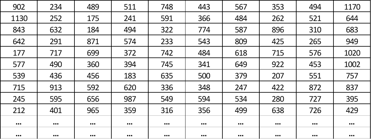
Create a histogram with interval = 100 days as shown:
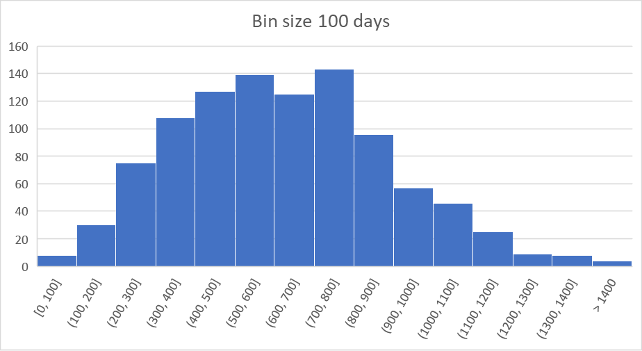
Suppose we want to estimate what percentage of the population would have failed by 300 days of operation—here's how we can do it:
There are 3 bars before 300 days. Its heights are 6, 31 and 74 respectively. Sum up the heights of these 3 bars, and we get 111 failures.
The total number of this sample is 1000 units. Therefore, the probability of a bearing failure is 0.111 for a 300 days operation.
Note that we can only query the probability of failures at 100, 200... at the resolution of the bin-size.
Let's overlay a function over the histogram as shown:
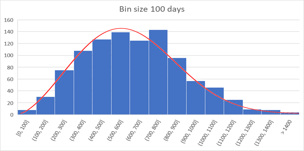
The function should have the following characteristics:
- The function profile averages out the value of each bar.
- The total area under this function is 1.
With this function, we can query the probability of failure at any time of interest. For example, you may query the probability of failure at 150 days by integrate the function from 0 to 150 days.
This function is called Probability Density Function. We denote pdf as f(t).
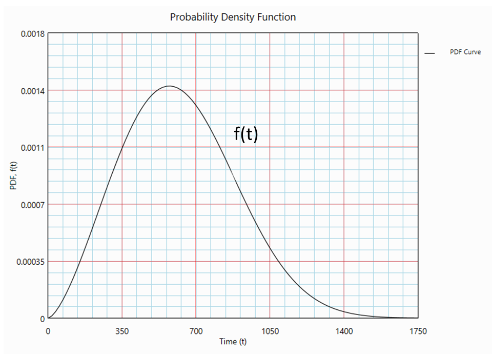
A Probability Density Function (PDF) is a mathematical function that describes the likelihood of a continuous random variable taking on a particular value. The probability that the variable falls within a specific range is found by calculating the area under the PDF curve over that interval. The total area under the entire PDF curve is always equal to 1, reflecting the certainty that the variable takes on some value within its domain.
Cumulative Density Function (CDF)
PDF provides a visualization of the distribution of the random variable, but trying read the area under the function up to a point in time can be a challenge.
CDF allows user to read the probability of failure at time t.
Most classical statistic books use F(t) to denote CDF. In reliability text book, Q(t) is used. CDF is also known as Unreliability function.
As shown in the figure below, we can read from CDF: Q(t=300 days) = 0.11
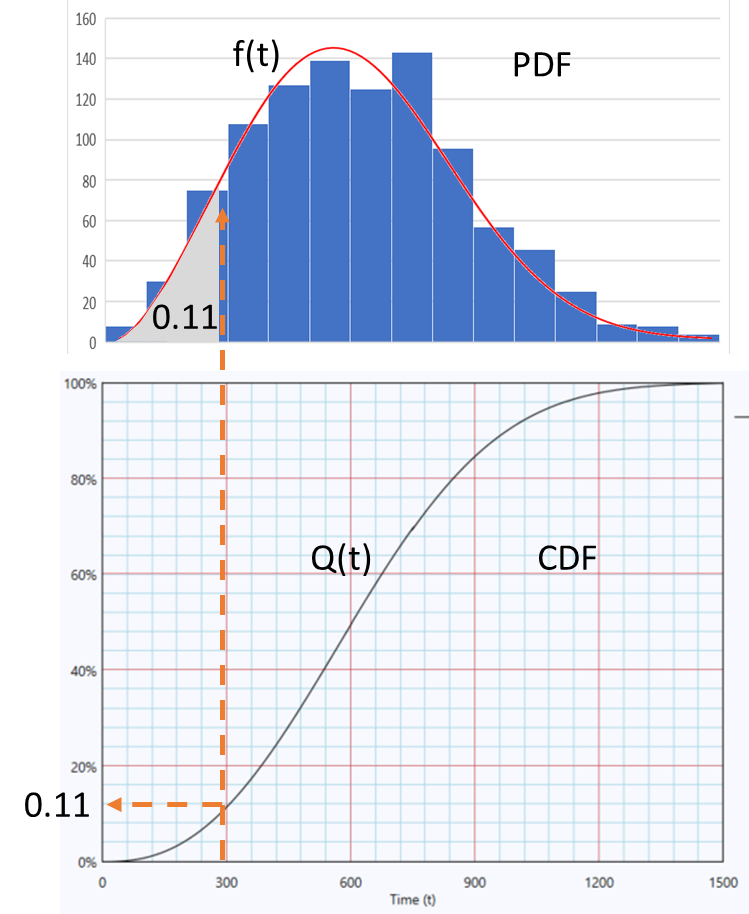
To read from the PDF, you must determine the area under the graph f(t) from t=0 to t=300 days. This is not a trivial task!
The CDF is the integral of the PDF.
Conversely, The PDF is the derivative of the CDF:
Reliability, Unreliability
The unreliability plot (CDF) allows users to read the probability at time t directly.
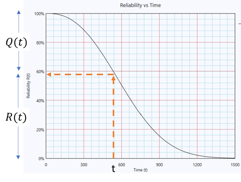
To obtain the Reliability at time t,
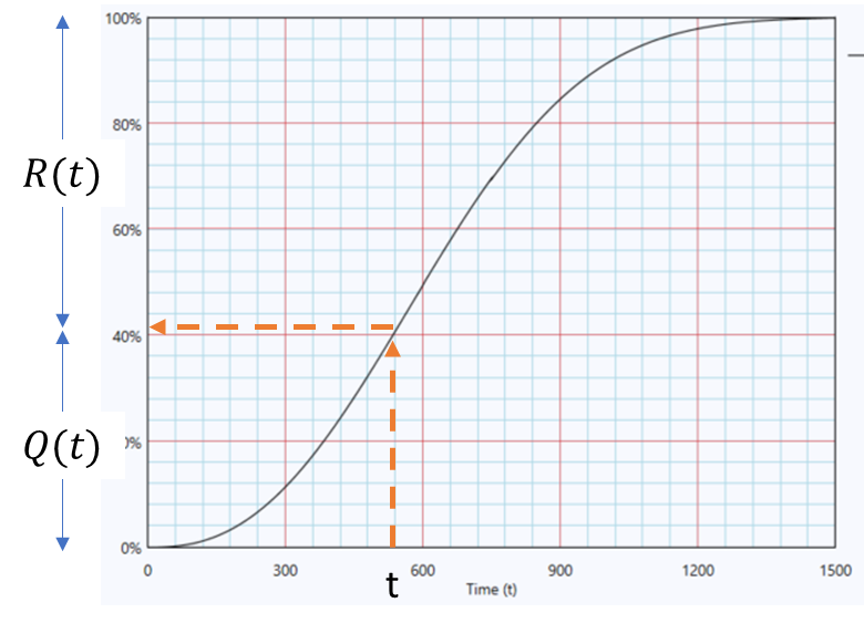
Using the equation, the reliability plot can be derived.
Failure Rate
Mathematically, failure rate at time t, λ(t), is defined as the probability of failure per unit time, given that the population have survived till time t.
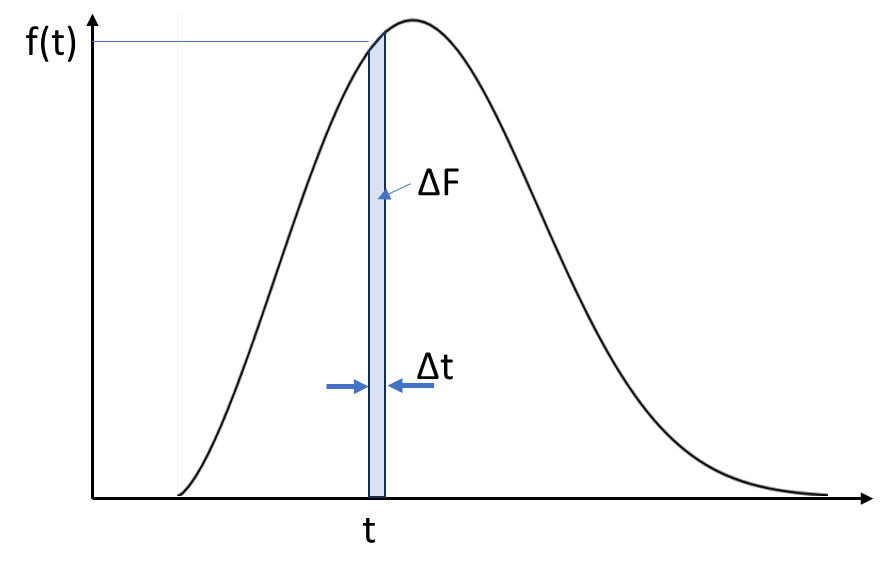
From definition,
where N(t) is the number of survivals at t, and is the initial population size.
Condition Reliability
Conditional reliability is the probability of a unit surviving a mission of 𝑡 duration, given that it has already accumulated an age of 𝑇.
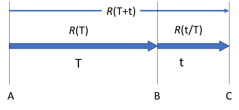
For an item to survival from point A to point C, it must have survived from A to B, and B to C. Hence,
Mean and Median
Mean time to failure (MTTF), is defined as:
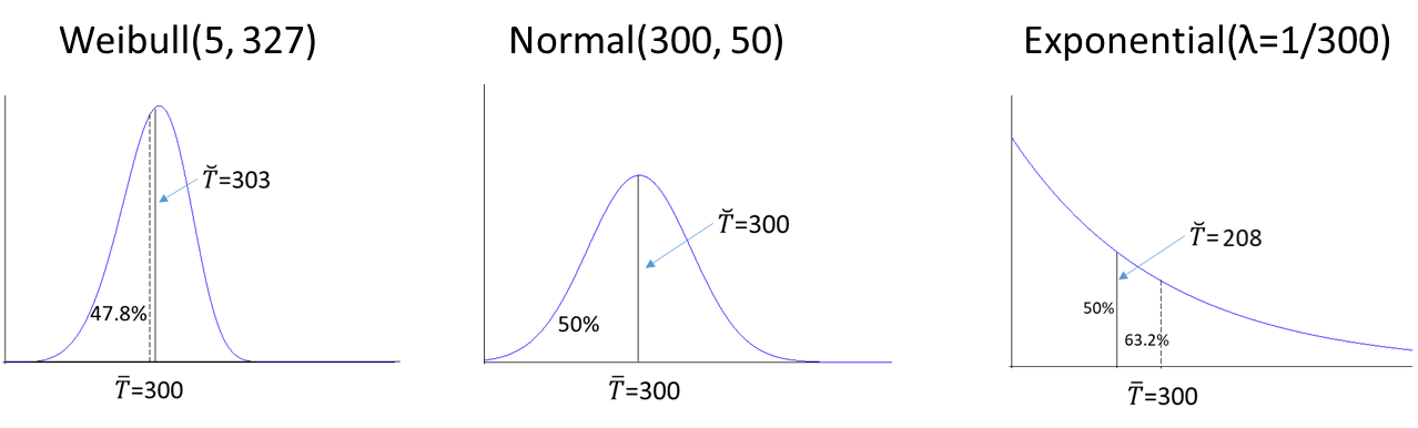
Median is the time by which 50% of the population fails.
Reliability Data Classification
In Life Data Analysis, reliability data falls into the following main types:
- Complete (Failure) Data: Each item is observed until failure. The exact failure time is known. This is the most straightforward type of data.
- Right-Censored Data (Suspension Data): The item did not fail during the observation period. We only know it survived up to a certain time. This is common in real-world testing or field data.
- Interval-Censored Data: The exact failure time is unknown but falls within a known time interval (e.g., checked periodically and found failed between two inspections).
- Left-Censored Data: The failure occurred before a known time, but the exact time is not observed.
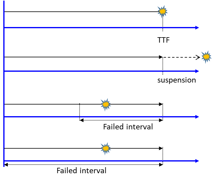
These data types are used together to estimate life distributions and reliability metrics.
Distribution Models
Distribution models are used to statistically describe the time until failure of components, systems, or products. These models help engineers and analysts understand the underlying failure behavior---whether failures occur randomly, increase with age, or follow a particular degradation pattern. By fitting a suitable distribution to observed failure data, one can estimate key reliability metrics such as failure rate, reliability over time, and mean time to failure. This allows for informed decisions in design, maintenance, warranty forecasting, and risk management, ultimately improving product reliability and operational efficiency.
Exponential (λ)
The exponential distribution is commonly used to model the time between random, memoryless events---particularly when the failure rate is constant over time. While simple, it's important and often serves as a baseline model in reliability and survival analysis.
Probability Density Function, PDF
The exponential 𝑝𝑑𝑓 𝑓(𝑡) is given by:
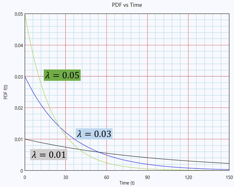
If is decreased, the Exponential distribution stretches to the right. The height decreases to preserve the total area under the probability density function (PDF), which must always equal 1.
Cumulative Density Function, CDF
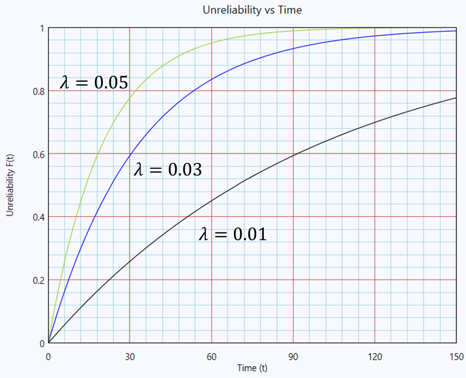
If is decreased, the Exponential distribution stretches to the right.
Failure Rate Function
The mean, , is given by:
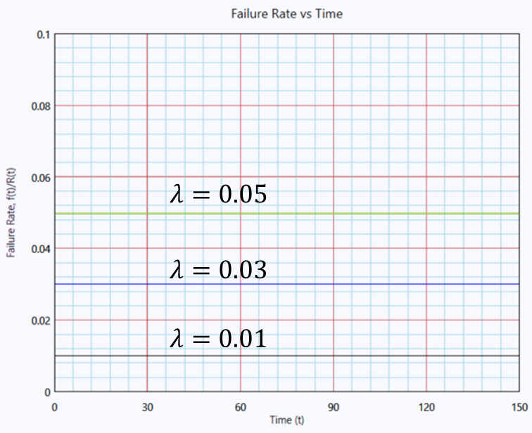
Mean Time to Failure (MTTF)
The mean, , is given by:
Median Life
The median life, is the time by which 50% of the population fails.
Weibull (β,η)
The Weibull distribution is commonly used to model time to failure data. Its flexibility allows it to represent a wide range of failure behaviors depending on its shape parameter β.
Probability Density Function, PDF
The Weibull PDF 𝑓(𝑡) is given by:
Effect of and on the PDF:
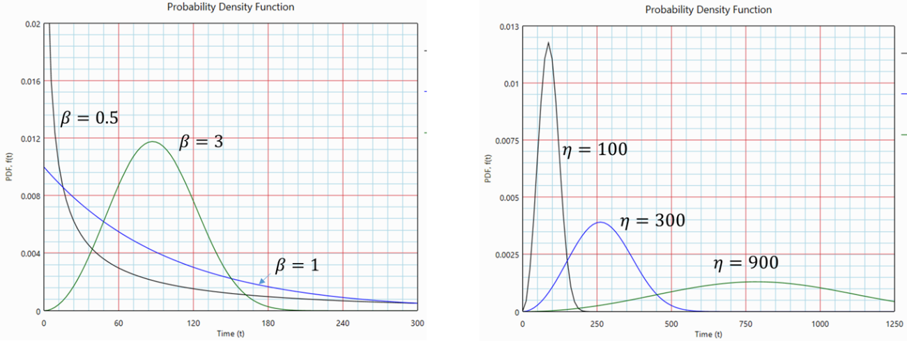
For : is Infinity at start, decays rapidly
For : Exponential shape
For : at start, peaks then decline
If 𝜂 is increased while 𝛽 remains constant, the Weibull distribution stretches to the right. The overall shape of the curve stays the same, but the peak height decreases to preserve the total area under the probability density function (PDF), which must always equal 1.
Cumulative Density Function, CDF
The CDF, also known as unreliability, is commonly denoted as Q(t) or F(t).
Effect of and on the CDF:
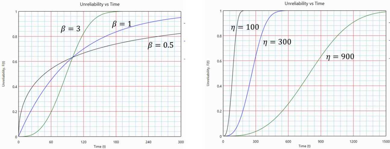
For : Rapid rise early, levels off slowly
For : Exponential shape
For : Shaped curve (slow start, then rapid rise)
If 𝜂 is increased while 𝛽 remains constant, the CDF curve stretches to the right. The overall shape of the curve stays the same.
Failure Rate Function
The failure rate function provides the percentage of failures occurring per unit time:
Substituting
and :
Effect of and on the failure rate function:
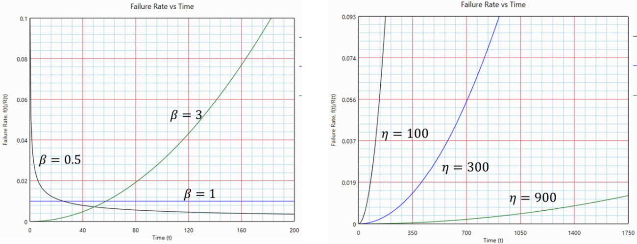
For : High failure rate initially, and decrease thereafter. Ideal for modelling infant mortality
For : Constant failure rate
For : S-shaped curve (slow start, then rapid rise)
Decreasing shifts failures earlier, increasing the failure rate at the same time t.
Mean Time to Failure (MTTF)
The mean, , of the Weibull pdf is given by:
Where
Median Life
The median life, is the time by which 50% of the population fails.
Normal (μ,σ)
The normal distribution is a symmetric, bell-shaped probability distribution that is widely used in statistics. In life data analysis, it's used less frequently than Weibull or lognormal because it allows negative values, which are not realistic for time-to-failure. However, it can still be appropriate in certain cases---particularly when variability is low and failures are clustered around a central value.
Probability Density Function, PDF
The Normal PDF 𝑓(𝑡) is given by:
Effect of and on the PDF:
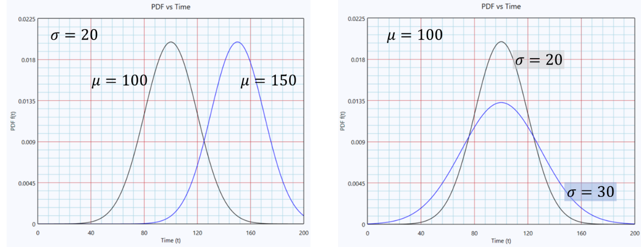
determines the center (mean) or location of the distribution.
controls the spread or dispersion of the data around.
Cumulative Density Function, CDF
Alternatively, Normal CDF can also be expressed using the standard normal CDF:
Where
: standard normal CDF
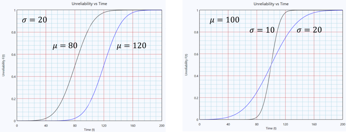
Effect of and on the CDF:
Failure Rate Function
The lognormal failure rate is given by:
where
Mean Time to Failure (MTTF) and Median Life
Since the normal distribution is symmetrical, the median is equal to the mean, and is the distribution parameter :
Lognormal (μ',σ')
The lognormal distribution is used to model failure times where the logarithm of the data follows a normal distribution. This distribution is particularly suitable for products or systems whose failure mechanisms are driven by the accumulation of damage or degradation over time---such as fatigue, corrosion, or chemical breakdown. The lognormal model produces a right-skewed curve, meaning most units fail around a certain time, but a few last significantly longer. It is characterized by a slow initial failure rate that increases over time, making it useful for modeling wear-out failure behavior where variability in time-to-failure is high.
Probability Density Function, PDF
The Lognormal PDF 𝑓(𝑡) is given by:
Where
: mean of the natural log of 𝑡 (log-location parameter)
: standard deviation of the natural log of 𝑡 (log-scale parameter)
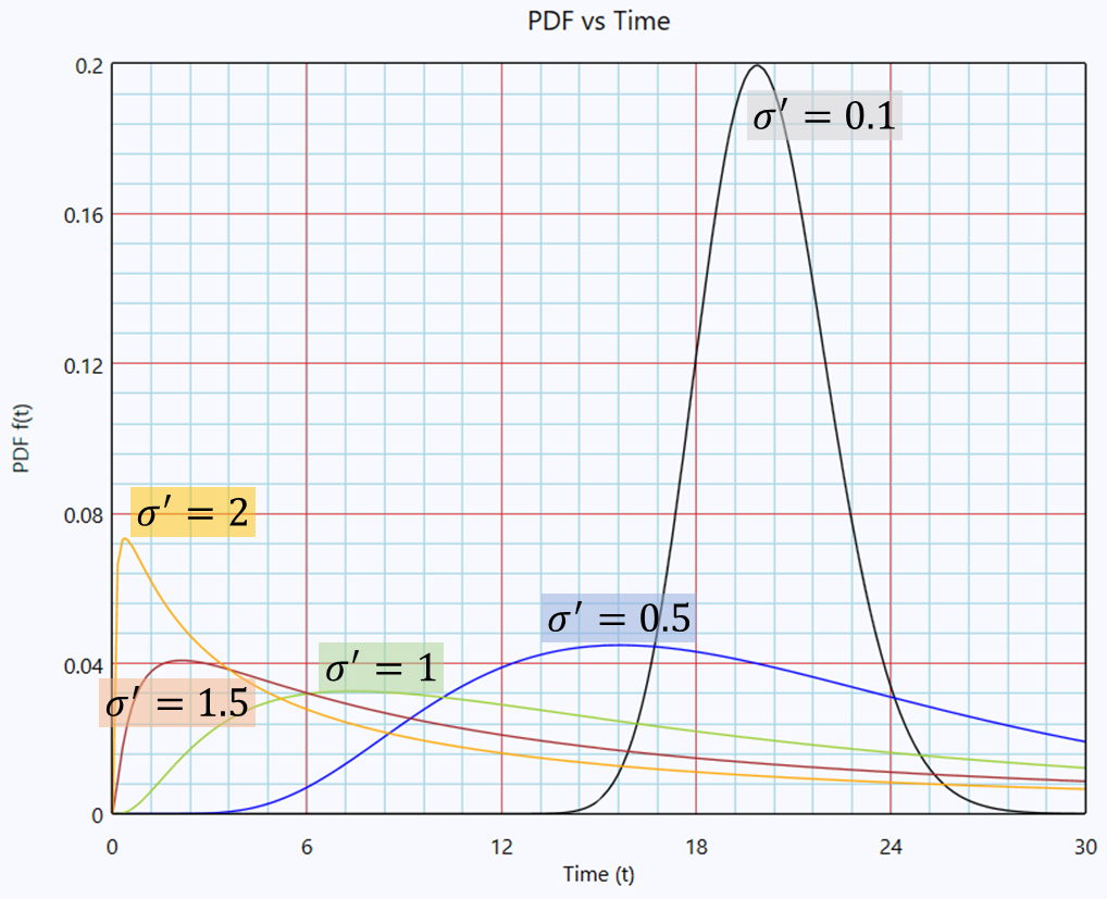
controls the spread and skewness of the distribution.
A larger value makes the curve flatter and wider, indicating a greater likelihood of very long lifetimes.
A smaller value (less than 1) results in a narrower and taller curve, meaning failures are more concentrated around the median.
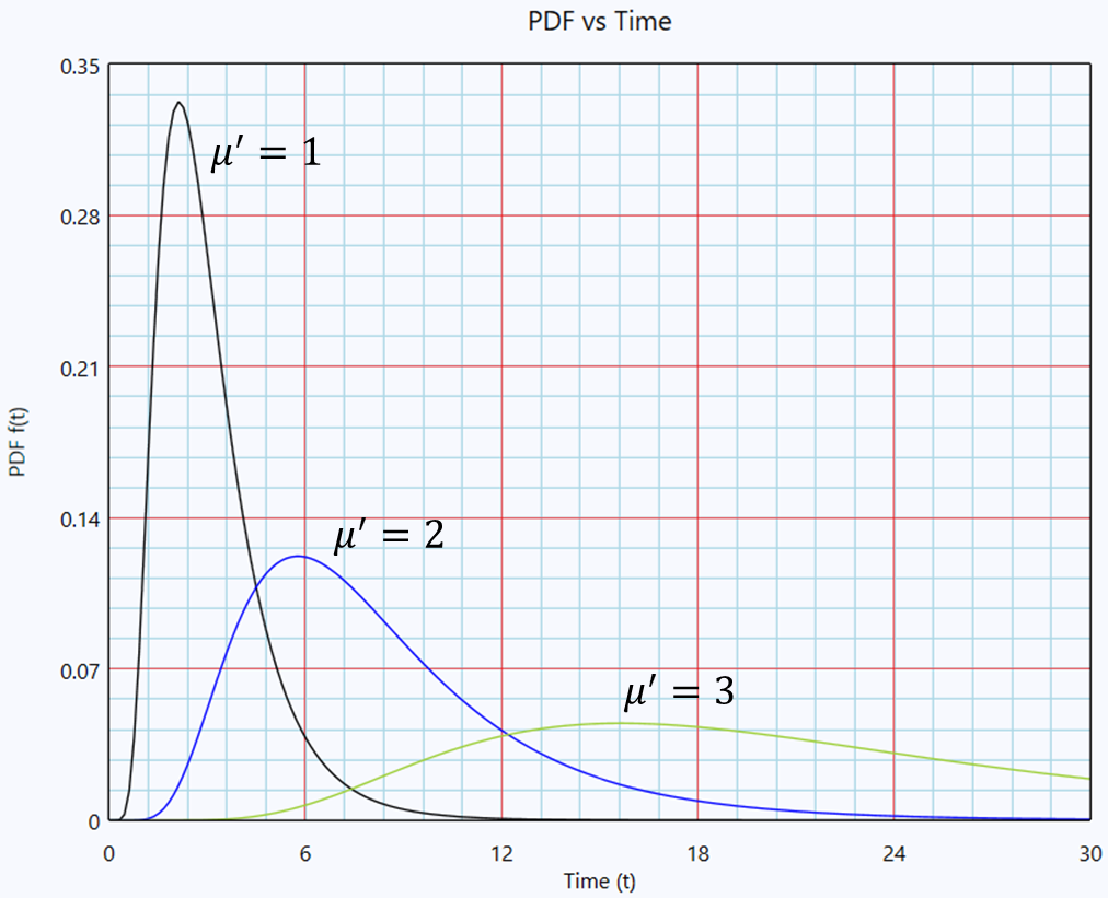
The parameter controls the horizontal positioning (time scaling) of the PDF but does not affect its shape.
Cumulative Density Function, CDF
Where
: mean of the natural log of 𝑡 (log-location parameter)
: standard deviation of the natural log of 𝑡 (log-scale parameter)
Alternatively, Lognormal CDF can also be expressed as:
Where
: standard normal CDF
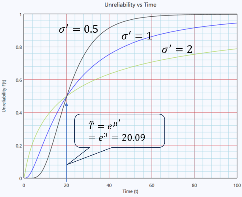
A larger stretches the CDF horizontally, indicating that failures are spread out over a wider range of times.
A smaller compresses the CDF and makes it steeper, meaning that failures are more concentrated within a narrower time window.
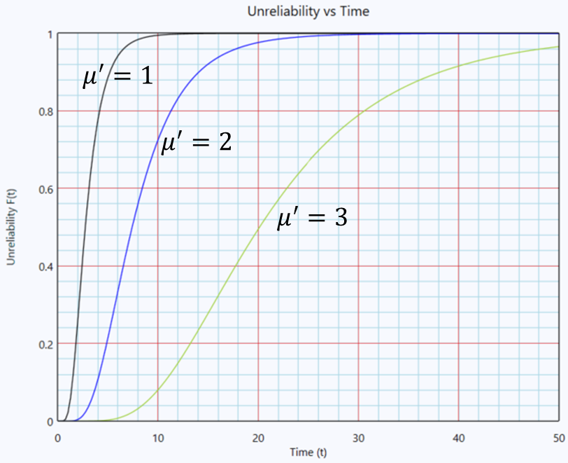
The parameter controls the horizontal positioning (time scaling) of the CDF but does not affect its shape.
Failure Rate Function
The lognormal failure rate is given by:
where
Mean Time to Failure (MTTF)
The mean, , is given by:
This integral evaluates to a known result in statistics:
Median Life
The median life, is the time by which 50% of the population fails.
Since ,
Parameter Estimation
The goal of parameter estimation is to determine the values of distribution parameters that best characterize a given set of observed data.
The following sections describe two widely used methods for this purpose: Probability Plotting and Maximum Likelihood Estimation (MLE). These techniques are commonly applied to fit parametric models such as the Weibull, lognormal, normal, and exponential distributions using sample data.
Probability Plotting
Probability Plot is a graphical method to estimate the parameters (e.g., mean, standard deviation, shape) of a theoretical probability distribution that best fits a given dataset.
The following dataset is used for illustration. {30, 40, 20, 50}.
We first sort the Failure Data: {20, 30, 40, 50}.
For each failure time ti, compute the cumulative probability qi using Cumulative Binomial equation.
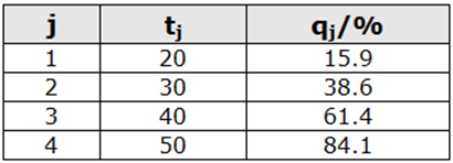
A cumulative probability is associated to each . The next step is to create the Probability paper. The X and Y axis are transformed such that the CDF appears as a straight line when plotted in this graph paper.
The following sections describe the concept of creating probability paper and solving for the various distribution (Exponential, Weibull, Normal and Lognormal) parameters.
Exponential Distribution
The cumulative distribution function (CDF) is:
Taking the natural log of both sides:
Hence, the plot of against t with form a straight line with slop -λ.
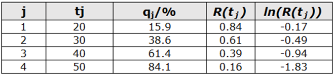
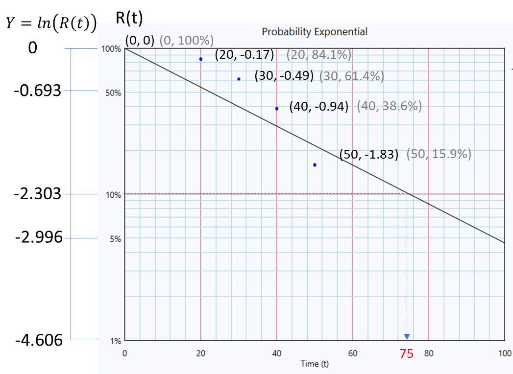
The co-ordinates (t, ln(R(t)) are plotted on the Probability-Exponential paper as shown.
Since R(t=0) is 1, the straight is forced to pass through
as shown.
To obtain the slop, pick a point on the fitted line know Y value to calculate the slop.
At Y = -2.303, the corresponding time is t = 75.
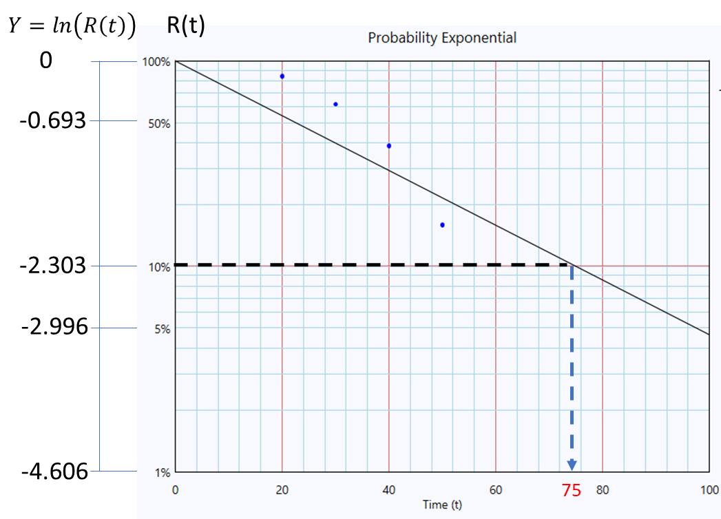
The Exponential parameter is:
per unit time
Weibull Distribution
For the Weibull distribution, the cumulative density function can be written as:
Linearize the equation: ,
where
Hence, the plot of Y against X with form a straight line with slop .
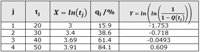
The co-ordinates (X, Y) are plotted on the Probability-Weibull paper as shown.
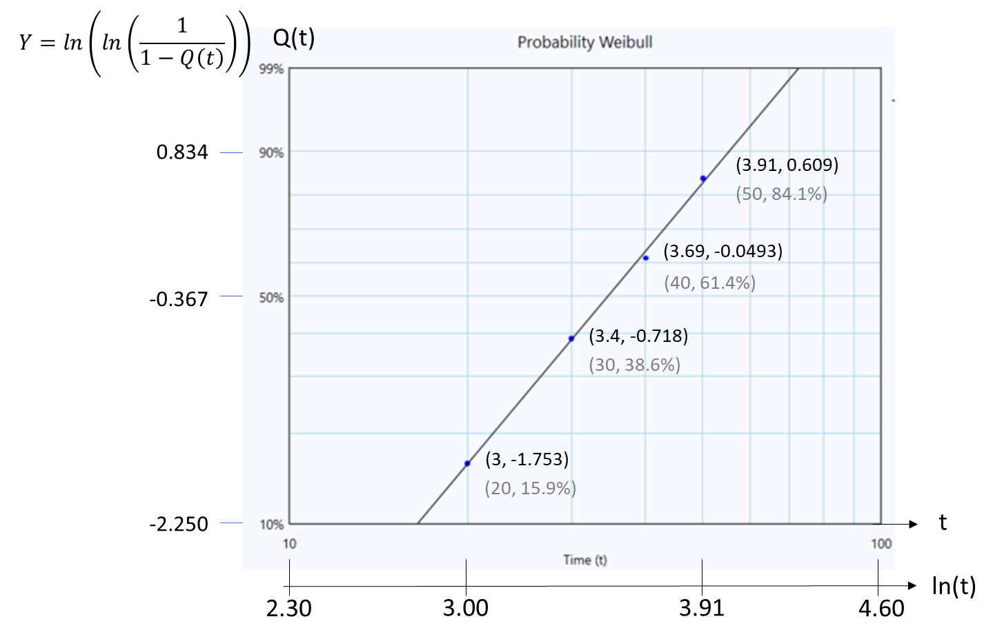
From Weibull CDF,
Let
Therefore, the time corresponding to Q=63.1% is the η value (=40), as shown in the graph below.
To obtain σ, pick two points on the fitted line with known Y-values (e.g., Y=0.834 and Y=-0.367), and calculate the slop.
For Z=0.834, cumulative probability Q(t)=0.9
For Z=-0.367, cumulative probability Q(t)=0.5
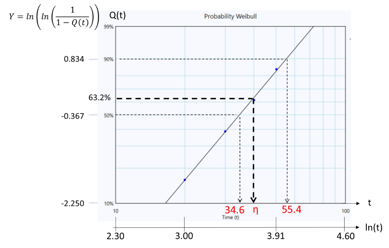
The is:
Normal Distribution
For the normal distribution , the cumulative density function can be written as:
where is the inverse of the standard normal CDF.
If we set as the Y-axis, and t (no transformation) as the X-axis, then the CDF of a Normal distribution will become a straight line with y-intercept = and slop = on this transform graph paper.
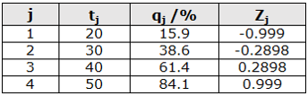
Now, we transform the cumulative probabilities Q(t) into standard normal quantiles (Z-values):
Note: You can use a standard normal table or a function like NORM.S.INV(Q) in Excel to get the Z values.
The co-ordinates (t, Z) are plotted on the Probability-Normal paper as shown.
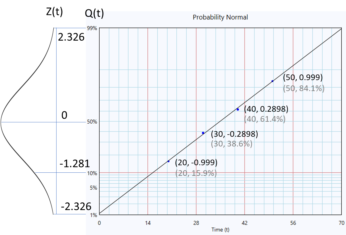
Mathematically, we can derive the mean and standard-deviation from the y-interception (), and the slop ().
For Normal distribution, . From the graph, .
To obtain σ, pick two points on the fitted line with known Z-values (e.g., Z=1 and Z=-1 ) and calculate the inverse of the slop.
For Z=1, cumulative probability Q(t)=0.841
For Z=-1, cumulative probability Q(t)=0.159
Note: You can use a standard normal table or a function like NORM.S.DIST(Z) in Excel to get the cumulative probability Q(t) values.
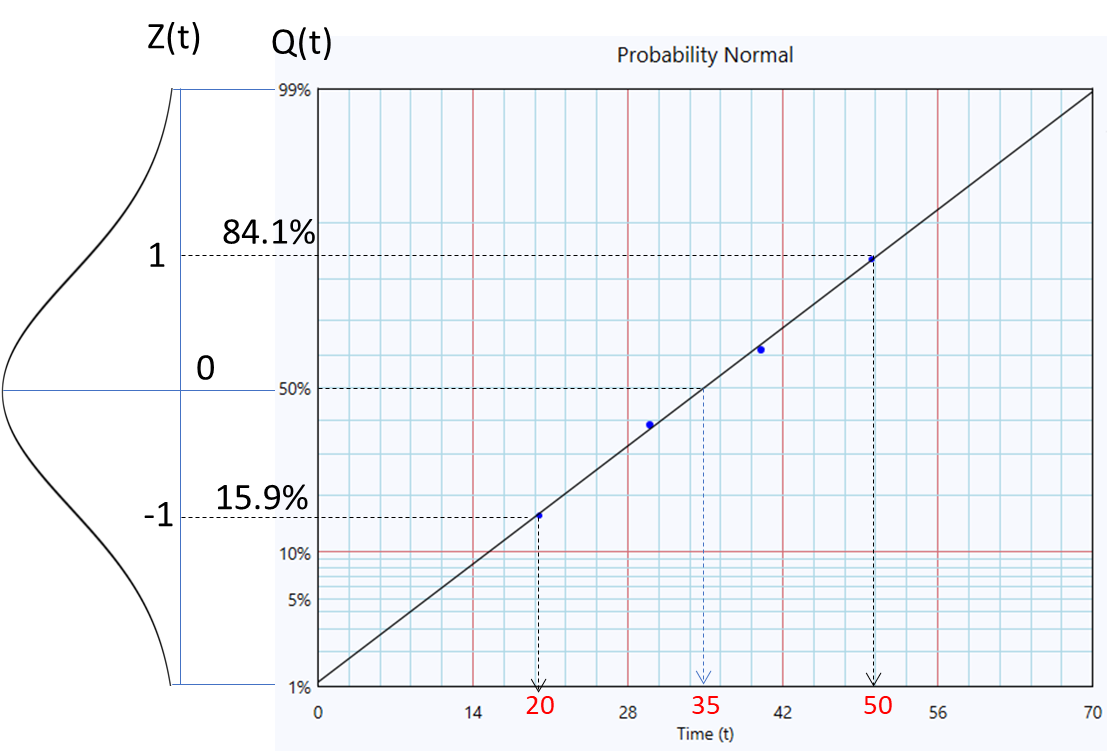
The Standard-deviation is:
Lognormal Distribution
If a variable t follows a lognormal distribution, then ln(t) follows a Normal distribution.
So, we simply take logarithms of the failure times and then plot them against standard normal quantiles.
For the Lognormal distribution , the cumulative density function can be written as:
where is the inverse of the standard normal CDF.
is the Mean of the log-transformed failure times.
is the Standard deviation of the log-transformed failure times.
If we set as the Y-axis, and ln(t) as the X-axis, then the CDF of a Lognormal distribution will become a straight line with a slope
Now, we transform the cumulative probabilities Q(t) on the Y-axis into standard normal quantiles (Z-values): , and the X-axis into ln(t).
Note: You can use a standard normal table or a function like NORM.S.INV(Q) in Excel to evaluate the Z value in the table below.
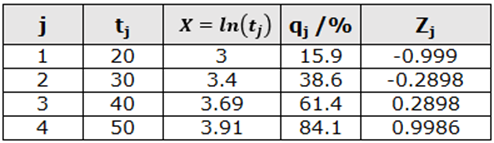
The co-ordinates (ln(t), Z) are plotted on the Probability-Lognormal paper as shown.
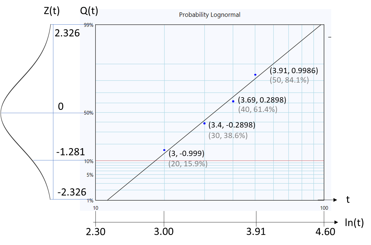
The log-mean (µ') occurs at Z=0, i.e., Q(t)=50%. At this point
The corresponding t for Q(t)=50% is 33.1, hence
To obtain σ', pick two points on the fitted line with known Z-values (e.g., Z=1 and Z=-1), and calculate the reciprocal of the slop.
For Z=1, cumulative probability Q(t)=0.841
For Z=-1, cumulative probability Q(t)=0.159
Note: You can use a standard normal table or a function like NORM.S.DIST(Z) in Excel to get the cumulative probability Q(t) values.
The corresponding t values at those points are 18.3 and 52.5 as shown.
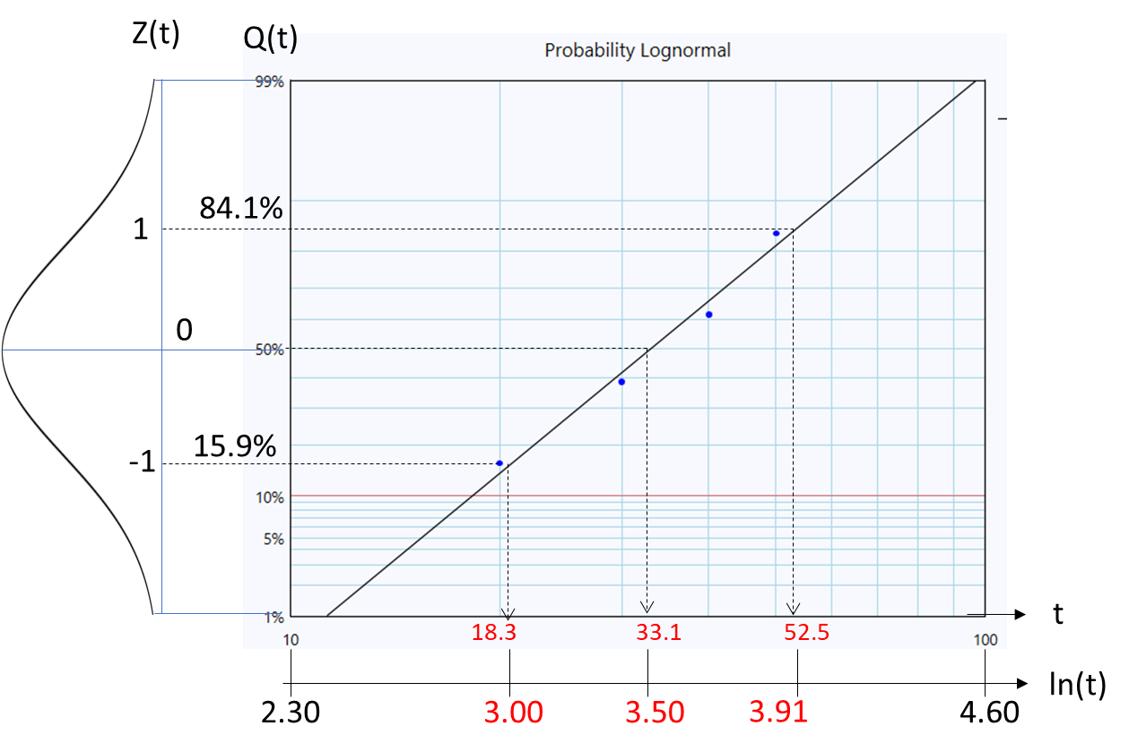
The Log Standard-deviation is:
Rank Regression
by fitting it to the observed data. The goal is to find the line that minimizes the sum of squared differences between the observed values and the values predicted by the line.
Rank Regression on Y
The RRY line (Rank Regression on Y) is a regression line that minimizes the horizontal distance (errors in the Y-direction) between each data point and the regression line.
It is used when we want to predict the time (e.g., failure time) for a given probability (e.g., 90% unreliability).
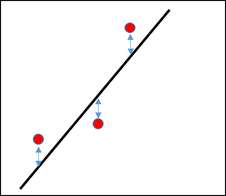
Given paired data points: (x1, y1), (x2, y2) ..., (xn, yn), and that the x-values are known exactly.
Where:
is the error term.
Rank Regression on X
The RRX line (Rank Regression on X) is a regression line that minimizes the horizontal distance (errors in the X-direction) between each data point and the regression line.
It is used when we want to predict the probability (e.g., 90% unreliability) for a given time.
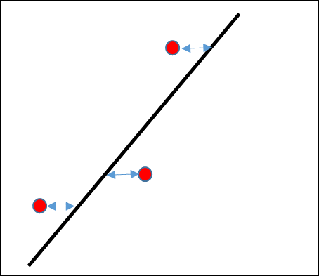
Given paired data points: (x1, y1), (x2, y2) ..., (xn, yn),
and that the y-values are known exactly.
To minimize the error in x-direction, regression of x on y is performed, i.e.,
Where:
is the error term.
Correlation Coefficient
One key concept in rank regression is the correlation coefficient, which serves as a measure of how well the chosen distribution fits the data.
The correlation coefficient ρ is defined as:
Where:
- and are the sample means of x and y,
- is the covariance,
- , are the standard deviations of x and y.
Interpretation
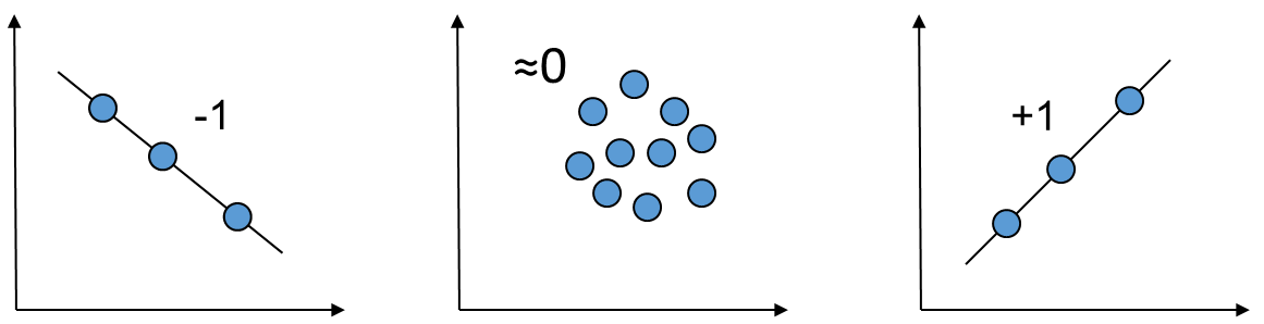
- The range is between -1 and +1.
- -1 is a perfect fit with negative slop.
- +1 is a perfect fit with positive slop.
Consider the following dataset:
{20, 30, 40, 50}.
The following plot shows the corresponding values when fitted to Exponential, Weibull, Normal and Lognormal model using Rank Regression on X (RRX).
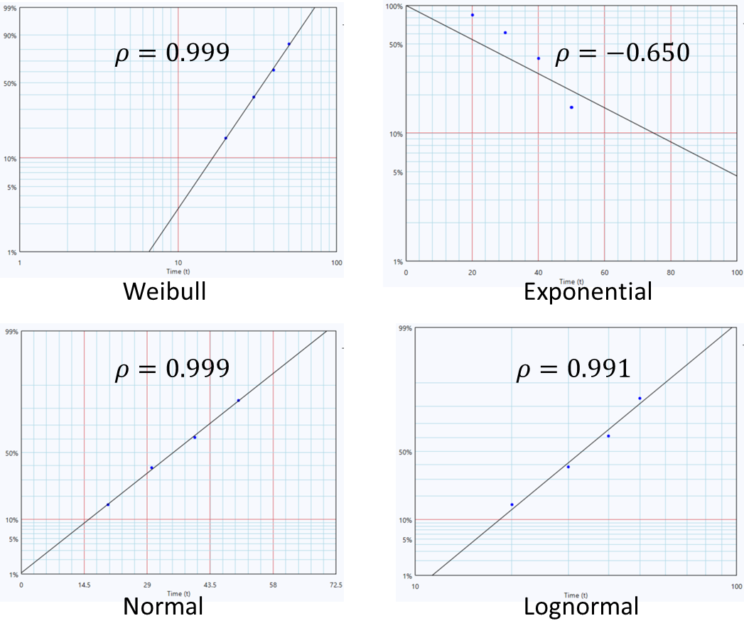
In the case of probability plot method (rank regression), the value can be used as an indicator of how well the chosen distribution fits the data.
Maximum Likelihood Estimations
Maximum Likelihood Estimation (MLE) is a statistical method used to estimate the parameters of a probability distribution by finding the values that make the observed data most probable under the assumed distribution. The key idea is to construct a likelihood function, which represents the probability (or probability density) of the observed data as a function of the unknown parameters. MLE seeks the parameter values that maximize this likelihood function.
Let:
: Probability density function (PDF) of the distribution (e.g., Weibull, lognormal).
: Cumulative distribution function (CDF).
: Reliability function (survival probability).
: Vector of unknown distribution parameters (e.g., shape and scale).
: exact failures at times .
: right-censored observations at times .
: interval-censored observations between and .
The complete likelihood function is given by:
Since maximizing the product is mathematically complex, it's easier to work with the log-likelihood:
MLE finds the parameter values θ that maximize this log-likelihood,Λ.
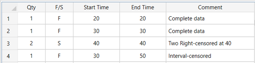
Let's consider fitting the following dataset to Weibull distribution using MLE analysis method:
PDF:
CDF:
Reliability:
Log-Likelihood Function:
Substituting Weibull functions:
The above Log-Likelihood is a function of .
Maximum Likelihood Estimation (MLE) determines the parameter values and that maximize the log-likelihood function .
Because this function is often nonlinear and complex, numerical optimization methods are required. The Weibull-Toolbox uses the Nelder--Mead optimization method to perform this estimation.
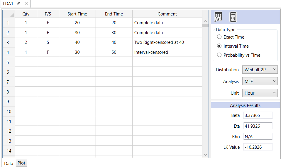
For this example, the β and η values are 3.37 and 41.9 respectively.
If these values are substituted back into the Log-Likelihood equation, we get:
In Weibull-Toolbox, the log-likelihood value is displayed under Analysis Results as the LK Value.
Suppose we fit the same dataset to several distributions---Normal, Lognormal, Weibull, and Exponential---and compare their LK Values:
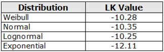
Since the Normal distribution yields the highest LK Value (i.e., the least negative), it represents the best fit among the options. In contrast, the Exponential distribution shows a significantly lower LK Value, indicating a poor fit to the data.
Confidence Bounds
Selecting a method. No single confidence-bound method is universally preferred. Fisher Matrix, likelihood-ratio, and simulation methods use different approximations and may produce different results, particularly when data are limited or heavily censored. The selected method should be appropriate for the data, fitted model, and engineering question.
Fisher Matrix Confidence Bounds
After fitting a Weibull model to failure dataset, we can quantify the uncertainty in the parameter estimates (, ) using Fisher Matrix Confidence Bounds (FMCBs) from which the variance for β and η can be derived.
Fisher Matrix Confidence Bounds on Parameter
We will demonstrate Fisher Matrix Confidence Bounds with Weibull distribution. The same concept is applicable to the other life distribution models.
The likelihood function for the 2P-Weibull distribution is:
- is the observed time for the i-th item,
- =1 for failures, and = 0 for censored data.
The log-likelihood function is:
Fisher Information Matrix for Weibull distribution
The Fisher Information Matrix I(β,η) quantifies the curvature of the log-likelihood function around the MLE point. It is defined as the negative expectation of the second derivatives:
Its inverse gives the covariance matrix of the estimates:
We assume that and are approximately normally distributed. It ensures that bounds for β and η remain strictly positive.
Shape parameter bounds:
can be approximated using the Delta Method as:
Hence,
For 90% confidence level, α=0.1, and
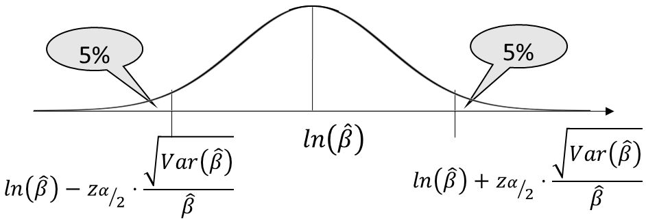
The 2-sided bound at confidence level α:
The scale parameter bounds:
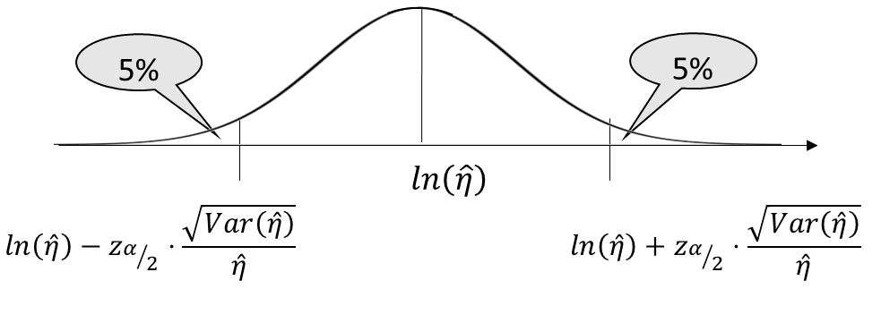
The 2-sided bound at confidence level :
Example:
A dataset {20, 30 ,40, 50} is fitted to a 2-P Weibull distribution using RRX. Find the 90% confidence bounds on the parameters.
The RRX solution: {beta=2.55, eta=39.9}
Fisher Information Matrix:
Covariance Matrix:
27.8
The concept of FM bound on an estimate can be summarized as follow:
1- Obtain the estimate through statistical analysis (In our case, MLE or RRX) and serve as our mean .
2- Derive the standard deviation σ, from Fisher Information Matrix.
3- Bound the estimate by the normal distribution with a standard normal quantile defining the confidence level.
Fisher Matrix Confidence Bounds on Time
Consider a dataset {20, 30 ,40, 50} that is fitted to a 2-P Weibull distribution. Find the 90% confidence bounds for the time interval where 10% of the population fails (unreliability Q=10%).
The RRX solution: {, }
Weibull CDF:
For ,
We bound a Normal distribution on time with mean = 16.5 as shown.
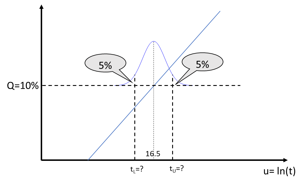
Since the x-axis is in natural-log scale Ln(t), the mean is actually ln(16.5).
We also need the variance Var(ln()) to completely define the Normal bound.
Let u =ln(t), the upper and lower bounds on u:
We have Var() and Var(), but not Var(). To derive Var(), we use Delta Method (Ref: Statistical Methods for Reliability Data by Meeker & Escobar, Appendix B, B2-Statistical Error Propagation-The Delta Method).
First, we need a relationship that expresses u in-terms of β and η.
From Weibull CDF
Linearize the equation:
Substitute
Using Delta Method:
)
Now, we can apply:
Since =>
= exp() = 33.5
= exp() = 8.13
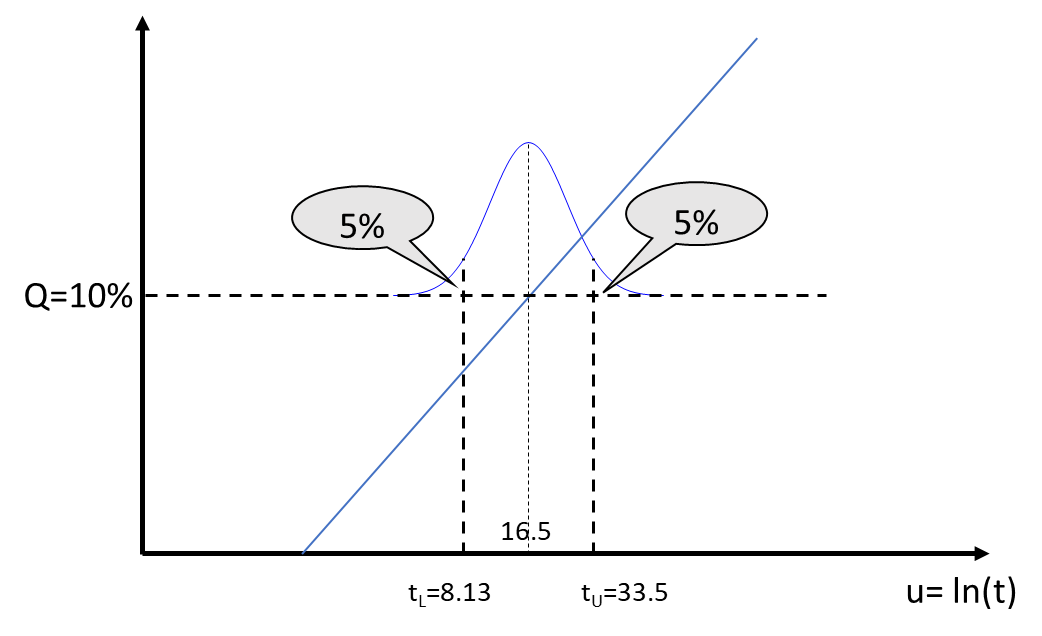
The 90% confidence interval on t is evaluated at Q=10% We can repeat for different Q value:
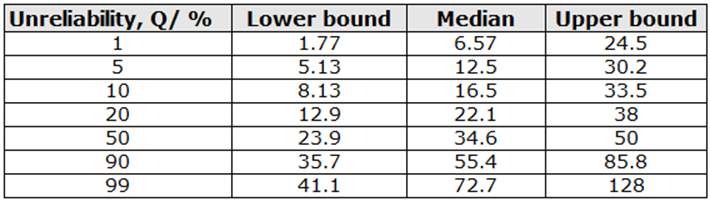
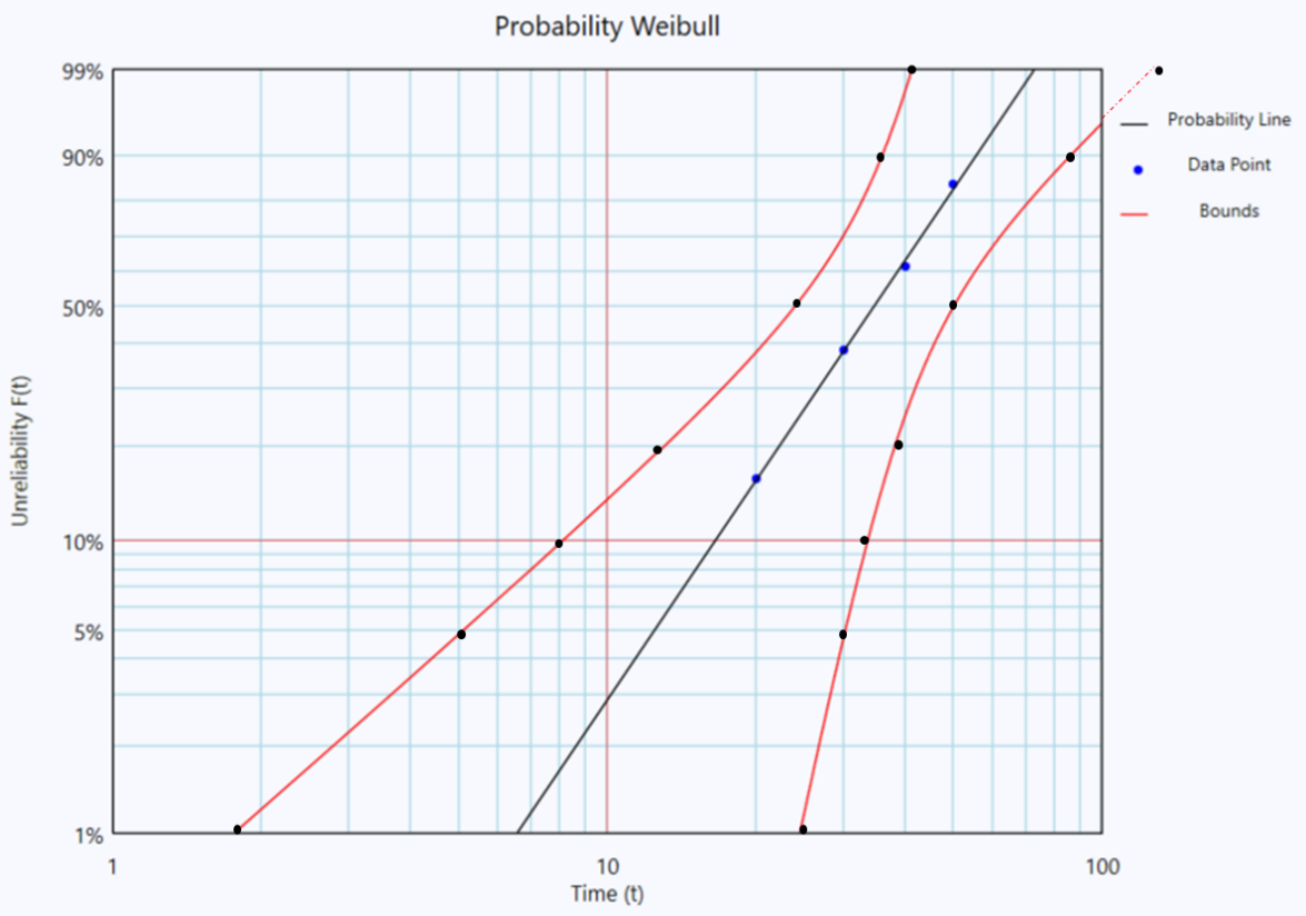
By joining the points on the probability plot, we obtain the confidence bounds as shown.
Fisher Matrix Confidence Bounds on Reliability
A dataset {20, 30 ,40, 50} is fitted to a 2-P Weibull distribution. Find the 90% confidence bounds for unreliability at time t = 20.
The RRX solution: {beta=2.55, eta=39.9}
From Weibull CDF:
For t=20, Q= 15.8%
We bound a Normal distribution on unreliability (y-axis) with mean = 15.8% as shown.
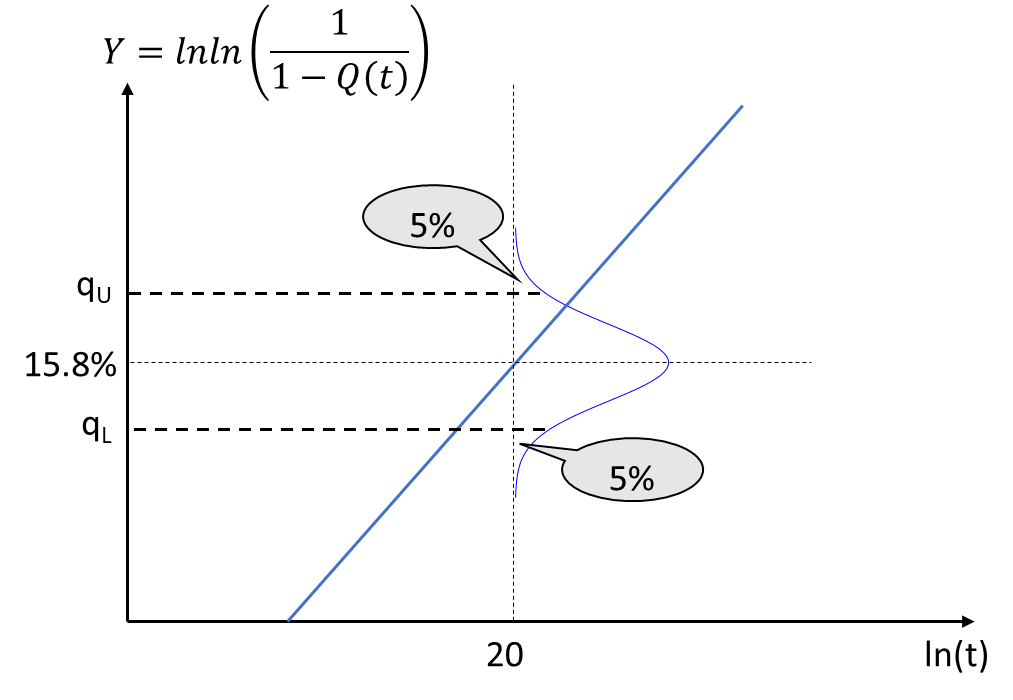
Since the y-axis is in double-log-reciprocal scale (), the mean is actually .
We also need the variance to completely define the Normal bound.
Let
, the upper and lower bounds on u:
We need a relationship that expresses in-terms of β and 𝜂, so that we can apply Delta Method to derive .
From Weibull CDF:
Linearize the equation:
Substitute
Applying Delta Method:
Now, we can apply:
Since =>
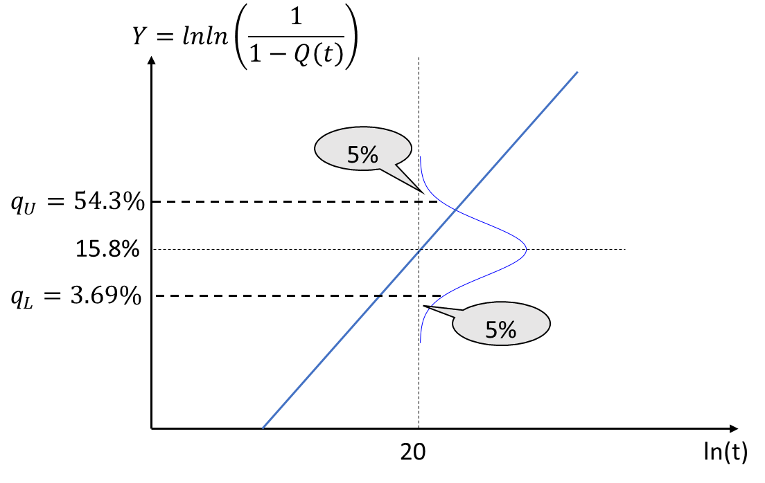
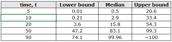
The 90% confidence interval on Q is evaluated at t=20. We can repeat for different t values, and overlay it on the probability plot.
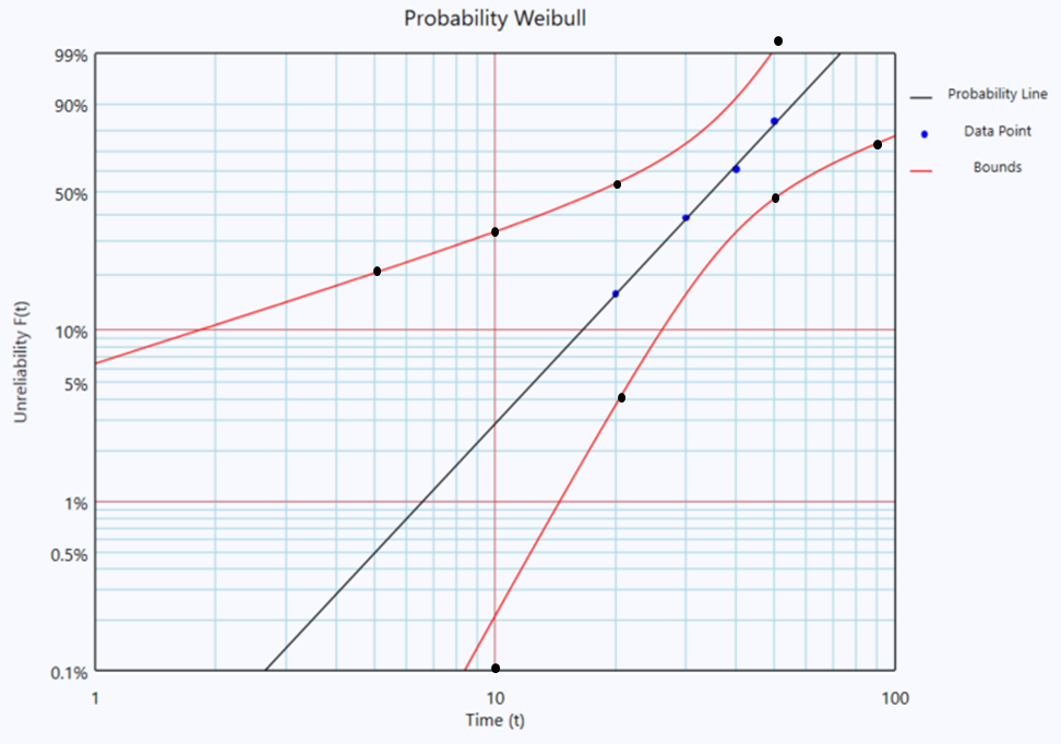
Likelihood Ratio Confidence Bounds
The Likelihood Ratio Principle
The Likelihood Ratio Confidence Bounds method is based on the likelihood ratio test.
The objective to estimate the confidence bounds on the β of Weibull distribution (that your dataset was fitted to).
Mathematically, the likelihood ratio statistic is:
: the likelihood function with eta value fixed at .
: the likelihood value evaluated at .
The likelihood function for the 2P-Weibull distribution is:
- is the observed time for the i-th item,
- =1 for failures, and = 0 for censored data.
The distribution of is not exactly known for small samples, but for large samples, Wilks' Theorem tells us it converges in distribution to a chi-square distribution with degrees of freedom equal to the number of parameters tested, 1 in this case.
The distribution of is constrained by the critical chi-square value 100(1−α)% confidence interval and one degree of freedom:
Hence, the bounds for β can be obtained by solving for maximum and minimum of β value that satisfy
Example:
A dataset {20, 30 ,40, 50} is fitted to a 2-P Weibull distribution. Find the 90% confidence bounds for beta using Likelihood Ratio Bound.
The MLE solution: { , }
Solve for the upper and lower beta values that satisfy:
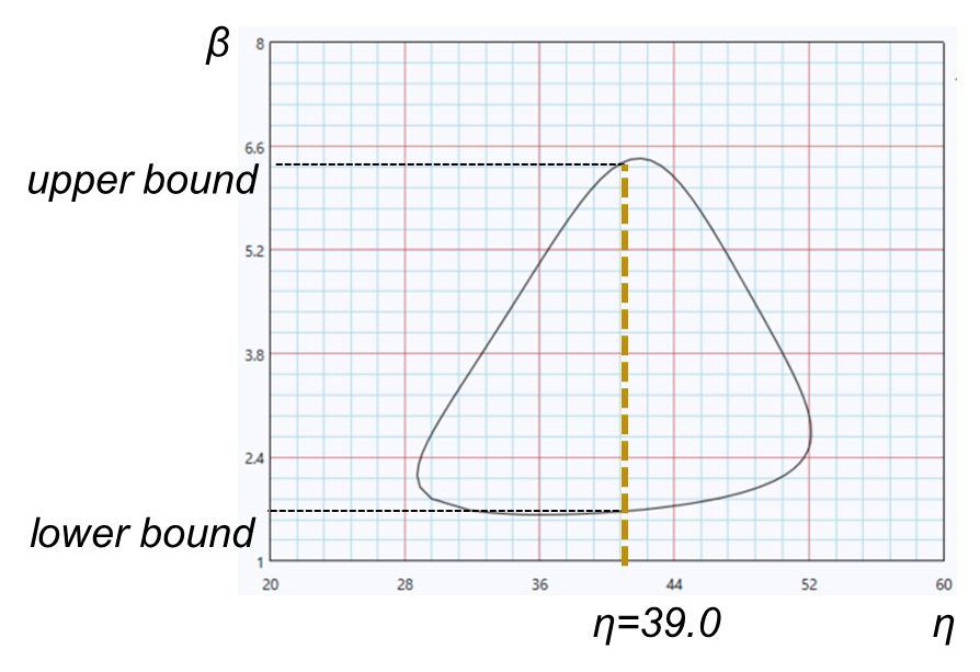
This defines the lower and upper confidence bounds for .
Similarly, bounds can be estimated.
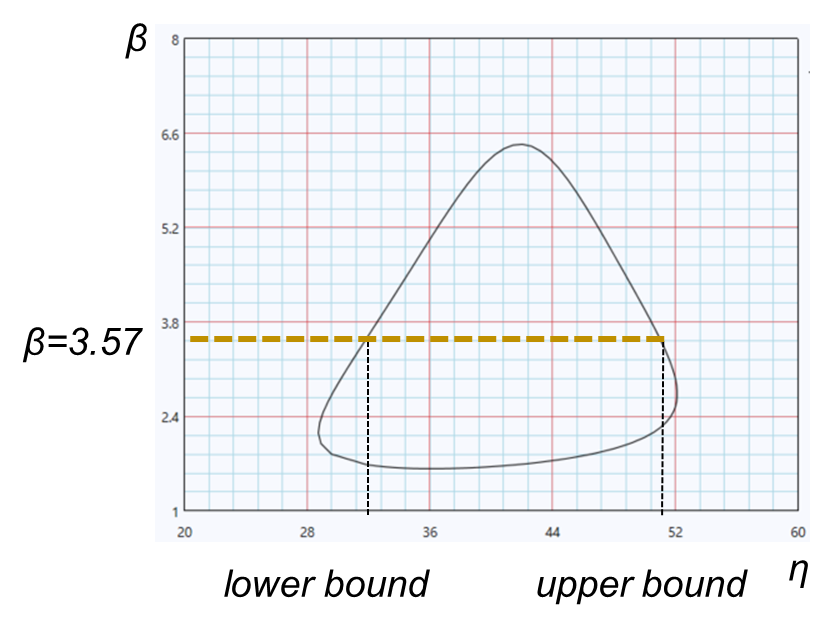
Confidence Bounds on Time
Consider the same dataset {20, 30 ,40, 50}, fitted to a 2-P Weibull distribution.
The B(10) life is t=20.8 unit time (or )
What is the 90% (2-sided) bounds?
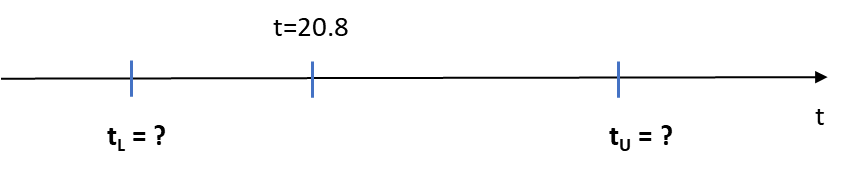
Mathematically, the likelihood ratio statistic is expressed in terms of t:
: the likelihood function with β value fixed at .
: the likelihood value evaluated at . This value is the same as .
is obtained by substituting
into .
For complete dataset,
where
and Q=0.1
Solve for maximum and minimum of t that satisfy
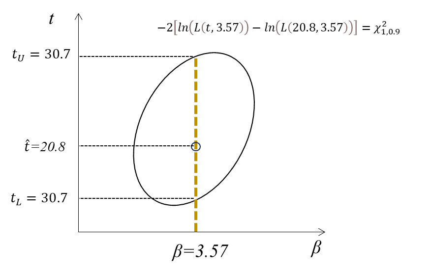
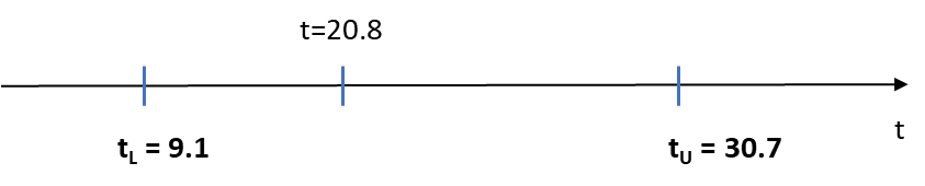
This can be interpreted as, 10% of the population is expected to fail between 9.1- and 30.7-unit time, with 90% confidence.
The 90% confidence interval on t is evaluated at Q=10%. We can repeat for different Q values:
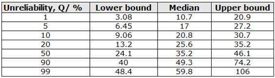
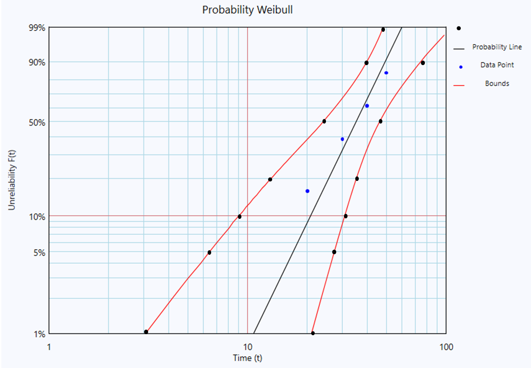
By joining the points on the probability plot, we obtain the confidence bounds as shown.
Confidence Bounds on Reliability
The procedure to obtain the reliability bound (for a given t) is the same as previous section.
The likelihood ratio statistic is expressed in-terms-of Q:
: the likelihood function with β value fixed at .
: the likelihood value evaluated at . This value is the same as .
is obtained by substituting
into .
For complete dataset,
where
Consider the same dataset {20, 30 ,40, 50}, fitted to a 2-P Weibull distribution.
At t=20, Q=8.81%. The aim is to estimate the lower and upper bonds of Q.

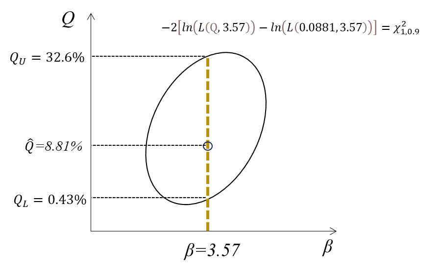

The 90% confidence interval on unreliability Q, is evaluated at t=20. We can repeat for different t values, and overlay it on the probability plot. Since the result is the same as Likelihood Ratio Bound on Time, we will not repeat it here.
Simulation Confidence Bounds
Simulation-based confidence bounds use repeated synthetic data sets to approximate the sampling uncertainty in fitted distribution parameters and derived reliability metrics. In this section, simulation refers to a parametric bootstrap: each synthetic data set is generated from the fitted life distribution rather than resampled directly from the observed values.
The resulting bounds can be calculated for distribution parameters, reliability at a specified time, or life percentiles such as B(10). They quantify uncertainty arising from the available sample, conditional on the selected distribution and estimation method. They do not account for an unsuitable distribution model, unrepresentative data, or incorrect assumptions about censoring.
Method
- Fit the original data. Select a life distribution and estimation method, such as Maximum Likelihood Estimation (MLE) or Rank Regression on X (RRX), and estimate the model parameters from the observed data.
- Generate parametric-bootstrap samples. Generate a sufficiently large number, , of synthetic life-data sets from the fitted distribution. Each synthetic data set should reproduce the original sample size and, where applicable, the original censoring or suspension scheme.
- Re-estimate the model. Fit every synthetic data set using the same distribution and estimation method used for the original data. This produces sets of fitted parameters and derived reliability results.
- Calculate percentile bounds. For each synthetic fit, calculate the quantity of interest—for example, reliability , B(10) life, or a distribution parameter. Sort the estimates and select the appropriate percentile for the required one-sided or two-sided bound.
Worked Example
The complete-failure data set {20, 30, 40, 50} is fitted with a two-parameter Weibull distribution. The objective is to construct a lower one-sided 90% pointwise confidence-bound curve on a Weibull probability plot using the parametric-bootstrap method.
1. Fit the original data
Using RRX, the fitted parameters are and .
2. Generate the parametric-bootstrap samples
Generate synthetic data sets from the fitted two-parameter Weibull distribution. Each data set contains four complete failure times, matching the original sample size and data structure. A larger value of can be used when smoother and more stable percentile estimates are required.
3. Re-estimate the parameters
Fit each synthetic data set with a two-parameter Weibull distribution using RRX. Each fit produces a new estimate of and and therefore a new fitted Weibull line.
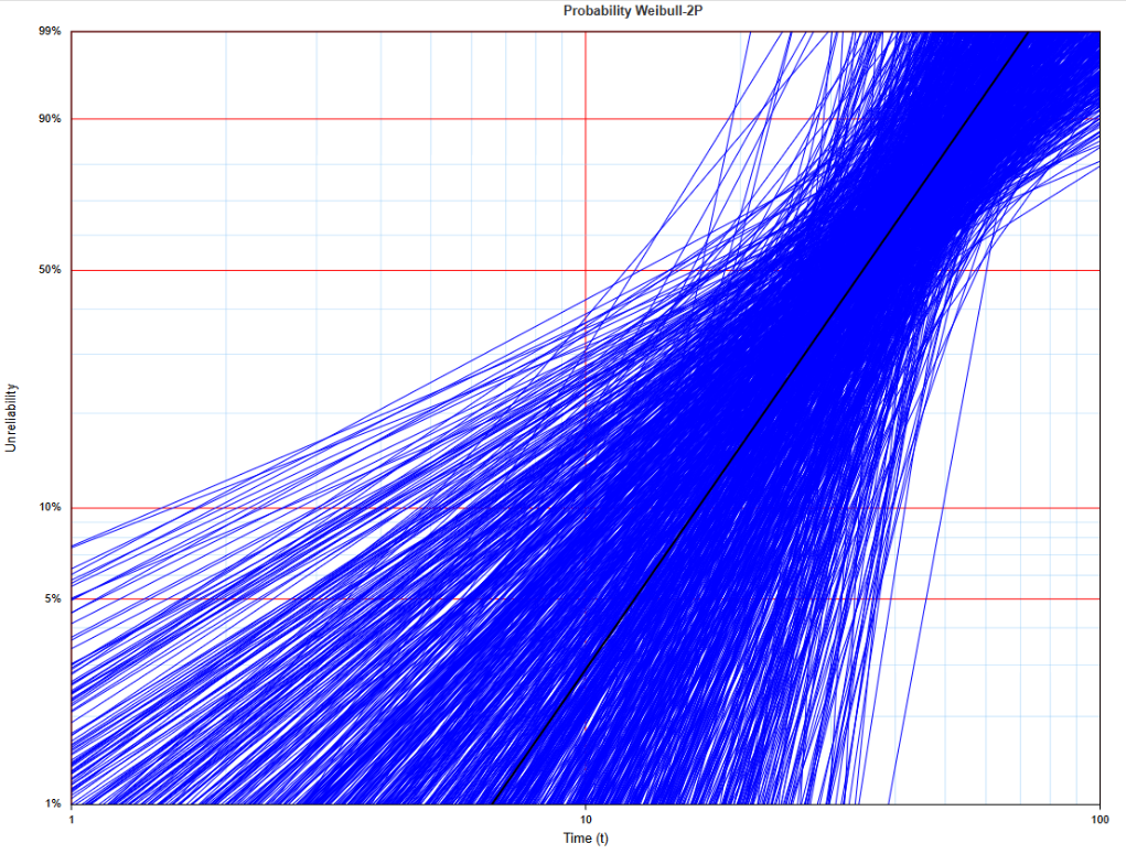
4. Estimate the lower one-sided 90% bound for B(10) life
Calculate B(10) for every bootstrap fit and sort the 1,000 estimates from smallest to largest. The lower one-sided 90% bound is the 10th percentile of this distribution—approximately the 100th ordered value when . In this example, the resulting lower bound is .
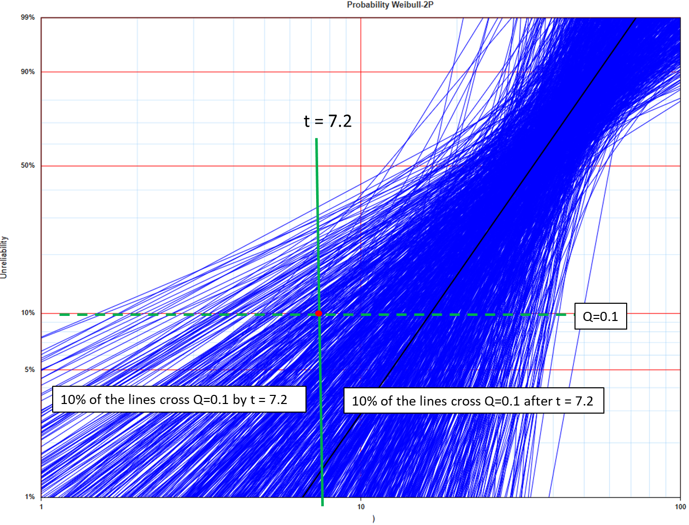
Repeat the calculation for B(1), B(2), …, B(99). At each unreliability level, select the 10th percentile of the corresponding bootstrap life estimates. Connecting these values produces the lower one-sided 90% pointwise confidence-bound curve. The word pointwise is important: the 90% confidence level applies separately at each unreliability level; it does not mean that the entire fitted distribution is contained within the curve with 90% confidence.
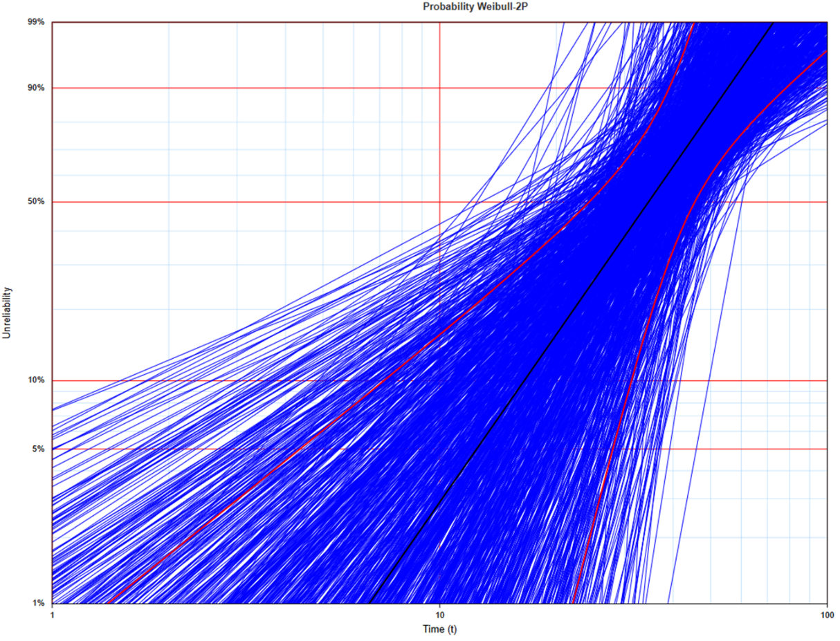
Figure 66 shows the lower and upper one-sided 90% bounds displayed by FreeWeibull.com. At each unreliability level, the lower curve is the 10th percentile and the upper curve is the 90th percentile of the bootstrap life estimates. The region between these curves therefore contains the central 80% of the bootstrap estimates and is equivalent to a central two-sided 80% percentile interval. It should not be interpreted as a conventional two-sided 90% confidence interval, which would use the 5th and 95th percentiles.
Recurring Data Analysis
Introduction
While Life Data Analysis focuses on systems that experience a single failure—capturing either the failure time or the current non-failed age—Recurring Data Analysis addresses scenarios where systems may undergo multiple failures over time. This analysis is particularly relevant for repairable systems where understanding failure trends and reliability over time is required.
Motivation for NHPP Model
From a reliability standpoint, the Non-Homogeneous Poisson Process (NHPP) model is useful for analyzing repairable systems. Key motivations include:
• Identifying trends in system failure intensity.
• Support decision-making for maintenance and overhauls.
• Providing a statistical model for reliability simulations, and digital twin analyses in RAM studies via tools like AeROS.
NHPP with Power Law
The Non-Homogeneous Poisson Process (NHPP) with Power Law is commonly used to model repairable systems. It accounts for systems that may either improve (e.g., under development) or deteriorate (e.g., in the field) over time.
NHPP Assumptions
• Repairs return the system to an 'as-bad-as-old' condition (minimal repair).
• Time-to-first-failure follows a Weibull distribution.
• The system has an unlimited number of failure modes.
Statistical Formulation
For a Poisson distribution with an expected value of λ events in a given time interval, the probability of observing n events is:
If λ is constant, the process is called a Homogeneous Poisson Process. If the cumulative failure function (mean value function) follows a power law with time:
Then the failure intensity (rate of failure over time) is obtained by differentiating Λ(t):
The probability of the random variable N(t) being equal to n is given by:
The term 'failure intensity' is preferred here over 'failure rate' to distinguish it from the usage in life data analysis.
Survival Probability and Reparameterization
The probability that a system of age t survives to t+d, without failure is given by:
If we re-parameterized the intensity function to follow Weibull failure rate function:
We get:
This reinforces the interpretation that the time to first failure follows a Weibull distribution, while subsequent failures follow the NHPP model.
Parameter Estimation of the NHPP Model
To estimate the parameters λ and β of the NHPP model, we use failure data from k systems. Let each system q (q = 1, ..., k) start operation at time Sq and end at Tq. Nq is the number of failures observed in system q, and Xiq denotes the system age at the i^th^ failure.
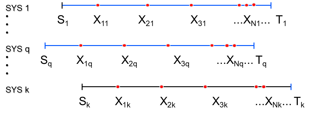
The maximum likelihood estimates for λ and β are given by:
Since these equations lack closed-form solutions, λ and β must be solved using iterative methods.
The value of provides insight into the system's behavior over time:
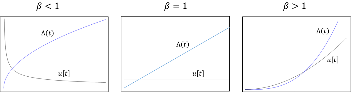
- : Failure intensity decreases with time (improving system).
- : Constant failure intensity (Homogeneous Poisson Process).
- : Failure intensity increases with time (deteriorating system).
Example: Pump Failure Data
Consider three pumps operating under similar stress conditions. Each pump experiences multiple failures over a defined operating period.
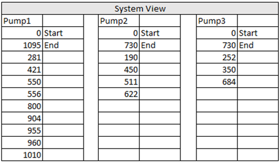
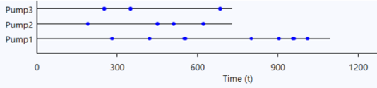
The cumulative failure records (in days) are entered into the RDA worksheet of the Weibull-Toolbox.
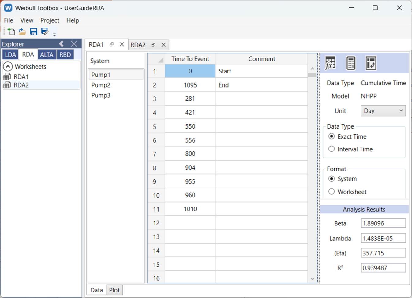
The MLE solution for the NHPP parameters is:
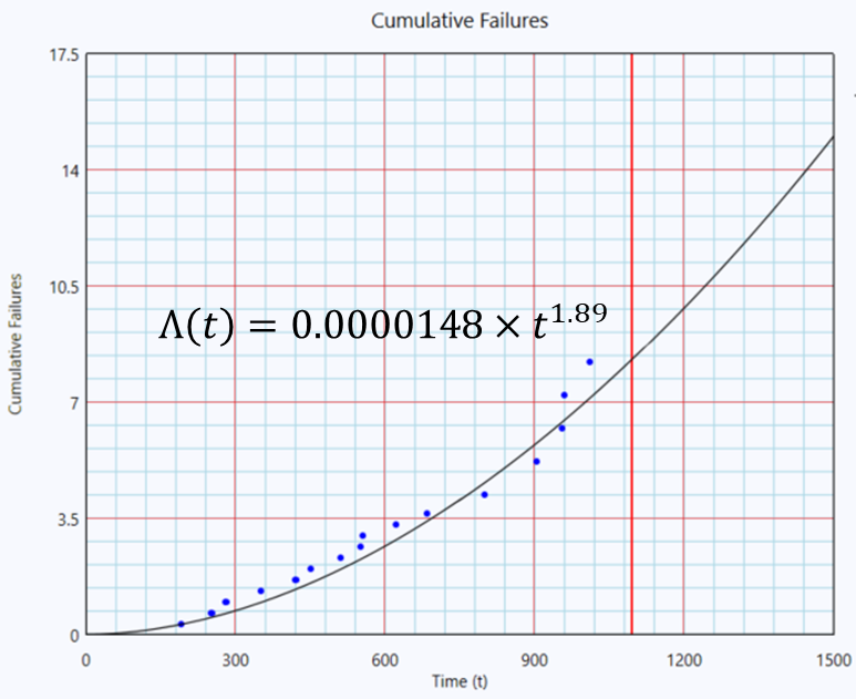
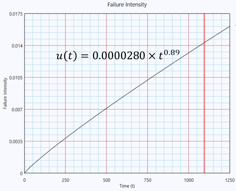
Using these parameters, the cumulative number of failures (mean value function) and the failure intensity function are plotted against time.
The Cumulative no. of Failure Function:
The Failure Intensity Function:
Confidence Bounds
Parameters estimated from recurring failure data are subject to sampling uncertainty. Confidence bounds provide a range of plausible values for the model parameters and for quantities derived from the fitted model, including the expected cumulative number of failures, failure intensity, and instantaneous MTBF.
The calculation described here uses the Fisher information matrix. The curvature of the log-likelihood near the maximum likelihood estimates provides approximate variances and covariance for and . Bounds on positive quantities are then formed on the logarithmic scale using the delta method, ensuring that all reported bounds remain positive.
Power Law NHPP Model
The expected cumulative number of failures by time , also called the mean value function, is
The corresponding failure intensity, or rate of occurrence of failures, is
The symbols used in this section are defined below.
| Symbol | Definition |
|---|---|
| Expected cumulative number of failures from time 0 to time | |
| Instantaneous failure intensity at time | |
| Scale coefficient; | |
| Shape parameter describing the trend in failure intensity; | |
| Number of repairable systems in the data set | |
| Start of the observation window for system | |
| End of the observation window for system | |
| Cumulative operating time of the th failure on system | |
| Number of observed failures on system | |
| Total number of observed failures, |
A single system observed from time 0 to time is the special case , , and .
Likelihood Function
Each system is observed over the window , and the systems are treated as independent NHPP processes. Under the NHPP assumptions, the log-likelihood of the combined failure history is
Natural logarithms are used throughout. When a system is observed from time zero, , the start-time terms involving powers and logarithms vanish in the limit and are omitted.
The maximum likelihood estimates and maximize this function and satisfy the score equations
As in the parameter-estimation section, these equations are solved iteratively, with start-time terms omitted when .
Fisher Information Matrix
The observed Fisher information is obtained from the negative second derivatives of , evaluated at the maximum likelihood estimates. Its elements are
The approximate covariance matrix of is the inverse of this information matrix. Let
Then
The covariance is retained whenever a bound depends on both parameters. These quantities are on the original parameter scale; the logarithmic scale is introduced when the bounds are formed.
Confidence Bounds on the Parameters
For a confidence level of , let be the standard-normal quantile appropriate for the selected bound type:
- Two-sided bounds use . For approximate 95% bounds, .
- Lower one-sided, upper one-sided, and both-one-sided bounds use . For approximate 95% bounds, .
Because and must remain positive, the normal approximation is applied to their logarithms using the delta method:
The bounds are
Both limits are calculated for every bound type. A two-sided display and a both-one-sided display show both limits. A lower one-sided display shows the lower limit, while an upper one-sided display shows the upper limit. One-sided and both-one-sided displays use the one-sided quantile.
Confidence Bounds on the Mean Value Function
At time , the fitted expected cumulative number of failures is
The required derivatives are
The approximate variance is
The pointwise bounds are
Dividing the variance by gives the delta-method variance of . At each selected time, the bounds describe uncertainty in the expected cumulative number of failures. They are not a simultaneous confidence band for the entire curve.
Confidence Bounds on Failure Intensity
The fitted failure intensity at time is
Its derivatives are
The approximate variance is
The bounds are
Confidence Bounds on Instantaneous MTBF
For a system whose failure intensity changes with time, the reciprocal of the failure intensity is reported as the instantaneous MTBF:
The reciprocal reverses the order of the limits:
This is a local quantity at time . It represents a long-term average time between failures only when , for which the failure intensity is constant.
Interpretation and Limitations
These bounds describe uncertainty in the estimated mean behavior of the NHPP model. They are not prediction limits for future failure counts. Future counts remain random around the mean value function according to the assumed Poisson process.
The Fisher-matrix method uses a local normal approximation to the likelihood surface. Its accuracy generally improves as the number of observed failures increases. With few failures, strongly correlated parameter estimates, or a markedly asymmetric likelihood surface, the approximation can be less accurate.
Confidence bounds also do not compensate for an unsuitable model. The assumptions and goodness of fit of the power-law NHPP model should be assessed before the bounds are used for prediction, maintenance planning, or economic decisions.
Time units must remain consistent throughout the analysis. Changing the unit of time changes the numerical value of , although the fitted physical failure process remains unchanged when the parameter transformation is performed correctly.
Optimum Overhaul (Economical Life)
In cases where β > 1, the failure intensity increases over time. While repairs may initially be more economical than overhauls, there comes a point where replacement is more cost-effective.
Let
= the overhaul time.
= corrective maintenance cost
= overhaul cost
The cost per unit time (CPUT) is defined as:
Where
To find the optimal , we differentiate CPUT with respect to and set the derivative to zero:
Solving yields:
For the pumps example with repair cost = $10,000 and overhaul cost = $50,000, and
The following shows the plot of CPUT vs Overhaul time.
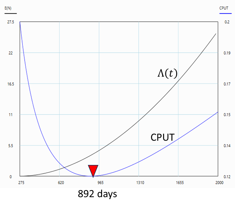
Note: For an optimal overhaul interval to exist, the following must hold:
• (failure intensity increases).
• Repair cost < Overhaul cost.
A beta value less than 1 indicates that the system's reliability improves over time; performing an overhaul may actually degrade its performance.
If the cost of repair exceeds the cost of an overhaul, the system should be replaced upon failure.
Accelerated Life Test Analysis
Introduction
Accelerated life testing (ALT) is used to obtain reliability information more quickly by testing units at stress levels above their normal use conditions. A life-stress relationship is fitted to the data collected at the accelerated conditions and used to estimate the life distribution at the intended use condition.
This section considers constant-stress ALT based on exact failure times, suspensions (right-censored observations), and interval-censored observations. Each observation must be associated with the stress level, or combination of stress levels, applied to that unit.
| Time to failure (hours) | |
|---|---|
| 350 K | 450 K |
| 200 | 10 |
| 350 | 15 |
| 425 | 30 |
| 820 | 45 |
| 1200 | 65 |
| 1250 | 70 |
| 1300 | 85 |
| 1600 | 130 |
| 2000 | 195 |
| 2100 | 300 |
Model Assumptions and Required Inputs
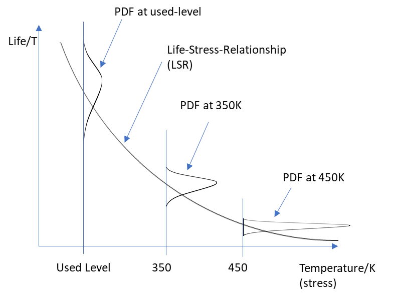
The extrapolation is meaningful only when the selected stresses accelerate the same failure mechanism that occurs under normal use. Under the usual scale-acceleration assumption, the distribution shape parameter remains constant across stress levels; stress changes the time scale but not the distribution family. Consequently, the absolute spread of failure times can increase as the life scale increases toward the lower-stress use condition, as illustrated above.
An ALT analysis therefore requires:
• A dataset containing the observed time, observation type, and associated stress value or values.
• A life distribution, such as Weibull, lognormal, or exponential.
• A life-stress relationship appropriate to the stress and failure mechanism.
• A defined use condition at which life or reliability will be estimated.
For one unknown stress effect, at least two distinct stress levels are required for mathematical identifiability. With stress variables, the design matrix must have full rank and therefore needs at least distinct stress combinations. In practice, additional stress cells and replication are normally needed to assess model adequacy and estimate uncertainty.
Likelihood for Censored ALT Data
Let denote the stress condition for observation . For exact failures, suspensions, and interval-censored observations, the combined log-likelihood can be written as:
where , , and are the numbers of exact failures, suspensions, and interval-censored observations, respectively. For interval observation , and are the lower and upper interval endpoints. The parameter values that maximize this log-likelihood are the maximum likelihood estimates (MLEs).
Arrhenius Life-Stress Relationship
The Arrhenius relationship is commonly used when temperature accelerates a thermally activated failure mechanism. It is written as:
Here, is absolute temperature in kelvin, and are model parameters, and is the distribution life scale at temperature . For a Weibull distribution, is the characteristic life ; for a lognormal distribution, is the median life.
Acceleration Factor
For a use temperature and an accelerated temperature , the acceleration factor is the ratio of life at the use condition to life at the accelerated condition:
Arrhenius Weibull Model
For a Weibull life distribution with a common shape parameter across stress levels:
The MLE solution consists of , , and .
Arrhenius Lognormal Model
For a lognormal life distribution with a common log-scale standard deviation across stress levels, define . Then:
The MLE solution consists of , , and .
Arrhenius Exponential Model
For an exponential life distribution, is the mean time to failure and the failure rate is . Then:
The MLE solution consists of and . This model is equivalent to an Arrhenius-Weibull model with .
Inverse Power Law Life-Stress Relationship
The inverse power law (IPL) relationship is commonly used for non-thermal stresses such as voltage, load, pressure, or vibration when life changes approximately as a power of stress:
Here, is the stress level and and are model parameters. The direction of acceleration must be consistent with the fitted value of and the physical failure mechanism.
Acceleration Factor
For a use stress and an accelerated stress :
IPL Weibull Model
For a Weibull life distribution with a common shape parameter :
The MLE solution consists of , , and .
IPL Lognormal Model
For a lognormal life distribution with a common log-scale standard deviation :
The MLE solution consists of , , and .
IPL Exponential Model
For an exponential life distribution, is the mean time to failure and . Then:
The MLE solution consists of and . This model is equivalent to an IPL-Weibull model with .
General Log-Linear Life-Stress Relationship
The general log-linear (GLL) model represents life as a function of one or more transformed stress variables:
Here, is the vector of transformed stresses and are model parameters. Weibull Toolbox supports up to three stress variables.
Relationship to Single-Stress Models
For one stress variable, the GLL model becomes . The transformation selected for determines the life-stress relationship:
• gives the Arrhenius form, with and .
• gives the IPL form, with and .
• gives an exponential life-stress form.
Acceleration Factor
For use and accelerated transformed-stress vectors and :
General Log-Linear Model with Multiple Stresses
Consider an ALT experiment with temperature and voltage as stresses. Suppose temperature follows an Arrhenius relationship and voltage follows an inverse power law. The example data are shown below.
| F/S | Interval start | Interval end | Temperature (K) | Voltage (V) |
|---|---|---|---|---|
| F | 65 | 65 | 300 | 5 |
| F | 77 | 77 | 300 | 5 |
| F | 90 | 90 | 300 | 5 |
| F | 90 | 110 | 300 | 5 |
| F | 90 | 110 | 300 | 5 |
| S | 110 | 110 | 300 | 5 |
| S | 110 | 110 | 300 | 5 |
| S | 110 | 110 | 300 | 5 |
| F | 35 | 35 | 300 | 10 |
| F | 40 | 40 | 300 | 10 |
| F | 43 | 43 | 300 | 10 |
| F | 49 | 49 | 300 | 10 |
| F | 55 | 55 | 300 | 10 |
| S | 55 | 55 | 300 | 10 |
| S | 55 | 55 | 300 | 10 |
| F | 6.5 | 6.5 | 400 | 5 |
| F | 8 | 8 | 400 | 5 |
| F | 8.8 | 8.8 | 400 | 5 |
| F | 10 | 10 | 400 | 5 |
| F | 12 | 12 | 400 | 5 |
F denotes a failure observation and S denotes a suspension. Rows with different interval start and end times are interval-censored observations.
The stress variables are transformed as for temperature and for voltage.
| F/S | Start | End | V1 (K) | V2 (V) | X1 = 1/V1 | X2 = ln(V2) |
|---|---|---|---|---|---|---|
| F | 65 | 65 | 300 | 5 | 0.003333 | 1.609438 |
| F | 77 | 77 | 300 | 5 | 0.003333 | 1.609438 |
| F | 35 | 35 | 300 | 10 | 0.003333 | 2.302585 |
| F | 40 | 40 | 300 | 10 | 0.003333 | 2.302585 |
| F | 6.5 | 6.5 | 400 | 5 | 0.002500 | 1.609438 |
| F | 8 | 8 | 400 | 5 | 0.002500 | 1.609438 |
GLL Weibull Model
For a Weibull distribution with common shape parameter :
For stresses, the MLE solution consists of , and .
GLL Lognormal Model
For a lognormal distribution with common log-scale standard deviation :
For stresses, the MLE solution consists of , and .
GLL Exponential Model
For an exponential life distribution, is the mean time to failure and . Then:
For stresses, the MLE solution consists of . This model is equivalent to a GLL-Weibull model with .
Summary
An ALT analysis combines a life distribution with a physically appropriate life-stress relationship. The main analysis decisions are:
- Prepare the data, including the observation type and stress value or values for every unit.
- Confirm that the same failure mechanism is being accelerated across the test conditions.
- Select the number of stress variables and the transformation for each stress.
- Select the underlying life distribution, such as Weibull, lognormal, or exponential.
- Estimate the model parameters by maximum likelihood and evaluate whether the distribution and life-stress assumptions are adequate before extrapolating to the use condition.