Using Simulation to Plan a Reliability Test When the Life Distribution Is Uncertain

Sample-size planning for a reliability test does not begin from nothing. It requires an assumed population life distribution and a defined test strategy. When adequate failure data are unavailable, the initial model may have to come from engineering judgement rather than statistical estimation.

Useful inputs may include results from an earlier product version, comparable products, supplier information, preliminary tests, and knowledge of the failure mechanism. These inputs should be treated as planning assumptions—not as evidence that the reliability requirement has already been met.

Assume that a company manufactures a component and must determine how many samples are needed for a reliability test. The required reliability statement is:

Historical life data are not yet available, but the engineers can describe two plausible points on the population failure curve:

Here, Q(t) is the cumulative probability of failure by time t. The next question is whether these two engineering assumptions can be converted into a provisional distribution model.

Assume a two-parameter Weibull distribution. In the Life Data Analysis module at FreeWeibull.com, select the Probability vs Time data type and enter the two assumed probability points. This is different from analysing a time-to-failure dataset: the two inputs represent engineering judgement about the underlying population.

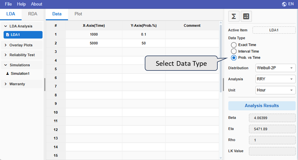
The resulting Weibull model has a shape parameter β = 4.06 and a characteristic life η = 5,472 cycles. For this fitted model, the nominal B(5) life is approximately 2,635 cycles and R(2,000) is approximately 98.34%. The point estimate therefore clears the target. However, the requirement is not based on the point estimate alone; it requires an 80% lower confidence bound.

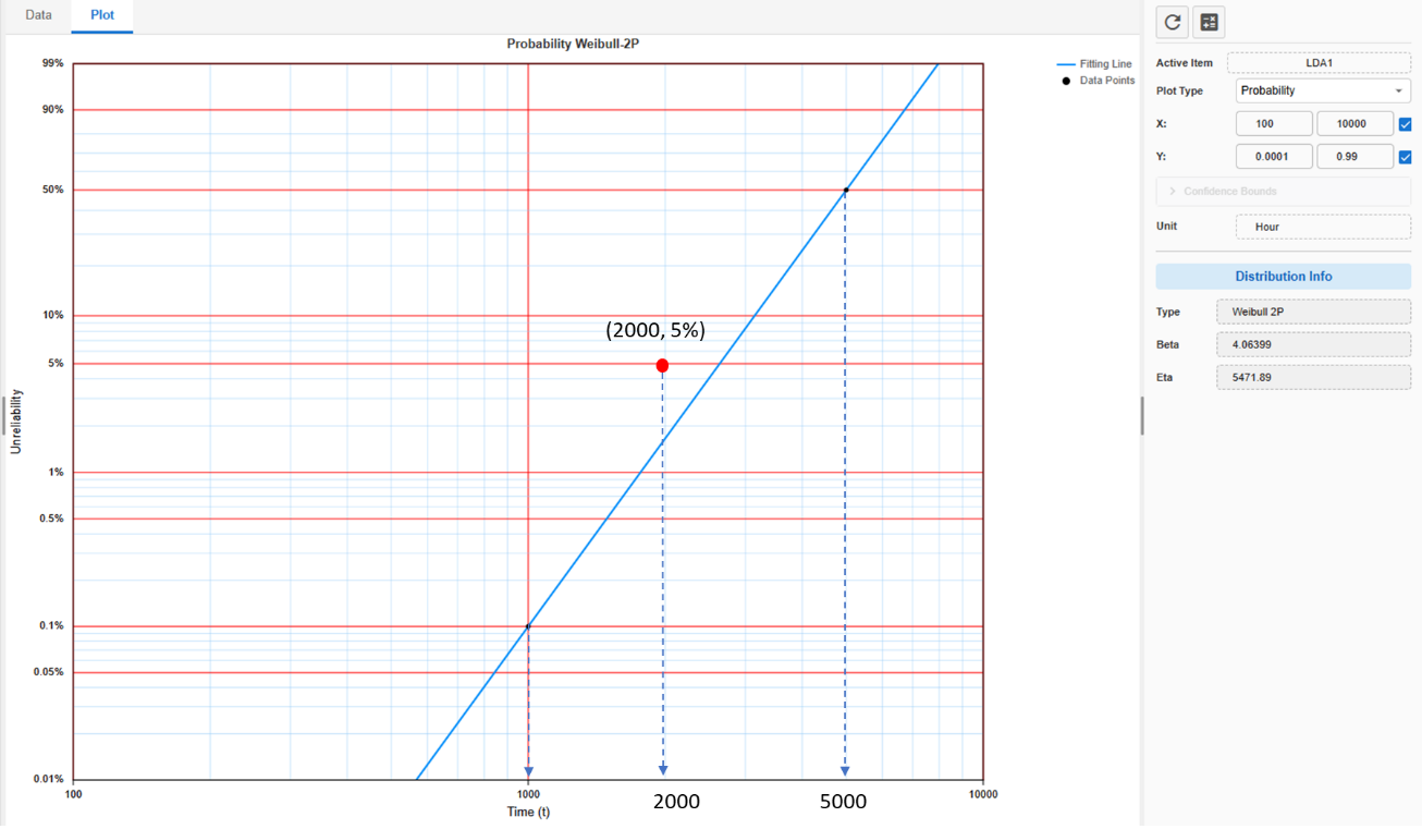
On the probability plot, the lower confidence bound on B(5) must lie to the right of the target point at 2,000 cycles. This distinction is important: a fitted line that clears the target does not by itself demonstrate the required confidence.

A confidence bound reflects the uncertainty in the estimated life model. Under the same test and analysis procedure, increasing the sample size generally narrows that uncertainty and moves the confidence bound closer to the fitted line. The bound is not determined by sample size alone; the number of failures, test conditions, assumed distribution, and estimation method also affect it.

For this illustration, simulated datasets are generated from the provisional Weibull model for different values of N. Each dataset is analysed using the same model and method, and the resulting 80% confidence bound is compared with the B(5) target.

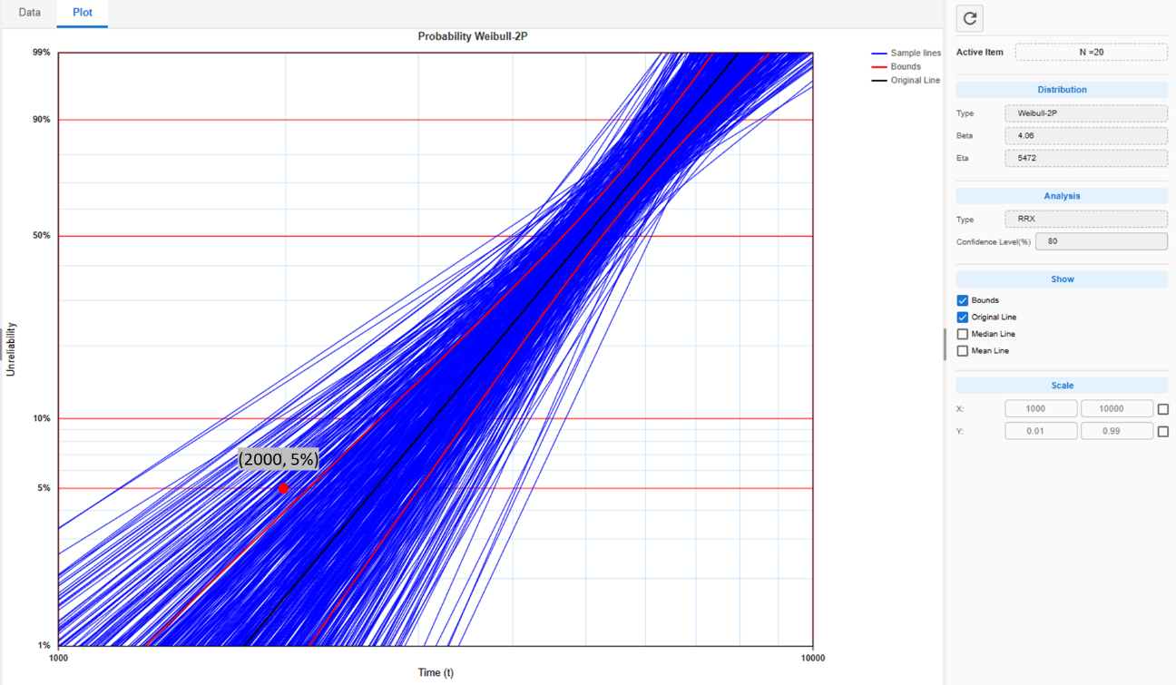
Start with N = 20. In the simulation shown in Figure 3, the 80% lower confidence bound remains to the right of the target point. Conditional on the assumed Weibull model and the simulated test conditions, 20 samples are sufficient.

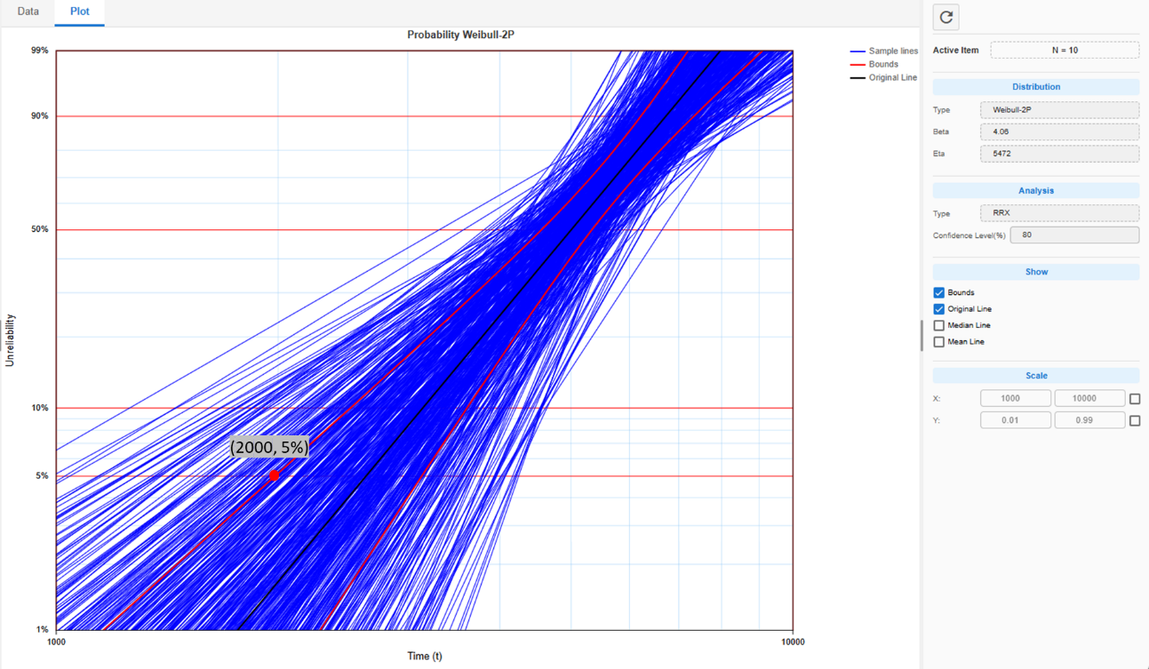
Next, reduce the sample size to N = 10. The confidence bound now passes through the target region, as shown in Figure 4. This suggests that a sample size around this level is near the practical boundary under the current planning assumptions.

The simulations suggest that 10 to 20 samples is a reasonable range for planning the reliability test. With N = 20, the 80% confidence bound remains to the right of the reliability target. With N = 10, it happens to pass through the target point.

This should not be treated as an exact threshold. A different simulation seed may move the confidence bound slightly to the left or right. More importantly, the assumed Weibull model is itself uncertain. Distinguishing precisely between 10, 12, or another nearby sample size would imply accuracy that the assumptions do not support.

The simulation helps determine a reasonable sample size; it does not guarantee the outcome. A test with 20 samples may still fail, while one with eight samples may pass. Only the actual test results can demonstrate whether the reliability requirement has been met.

• The result is conditional on the assumptions. The Weibull distribution and the two probability points are provisional engineering inputs, not observed evidence.
• The simulation should represent the actual test plan. The sample-size estimate is meaningful only when the simulation assumptions reasonably reflect how the test will be conducted and analysed.
• The test provides the evidence. Simulation can estimate the sample size and support a budget request, but only the observed test results can demonstrate whether the component meets the reliability requirement.

When historical life data are limited, simulation provides a disciplined way to move from engineering judgement to a testable plan. Its value is not that it removes uncertainty, but that it makes the assumptions visible, quantifies their consequences, and helps the engineering team decide how much testing is needed before making a reliability claim.