Introduction
Within maintenance organizations, historical failure data extracted from Computerized Maintenance Management Systems (CMMS) serves as a foundational data source for reliability analysis. This presentation highlights the challenges encountered when employing Life Data Analysis on recurring datasets, presenting an alternative statistical model, Recurring Data Analysis, tailored specifically for these scenarios.
Life Data Analysis
Life Data Analysis LDA is used to quantify the reliability of a population of items by statistically fitting its observed time-to-failure (TTF) data to some predefined distribution models. The statistical assumptions necessitate that the items are identical, and these items operate independently. These criteria are often abbreviated as IID (Identical and Independently Distributed).
These IID pre-requites imply that, when applying LDA to a population of items:
- Each sample has one observed value, either its age at "failure" or its current age while "non-failed".
- Every time-to-failure (TTF) data point must correspond to a distinct physical sample.
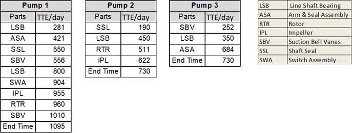
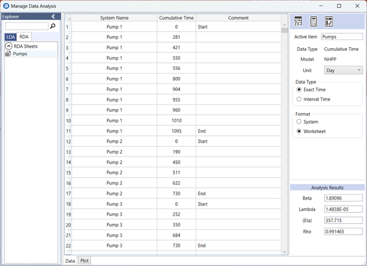
Consider the following failure data collected from a maintenance record, detailing the failure instances of three pumps operating independently under similar stress conditions. Pump 1 has functioned for 3 years, while pumps 2 and 3 have each operated for 2 years.
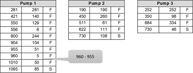
Following describes a common mistake: Take the time-between-failures for each system and fit a distribution!
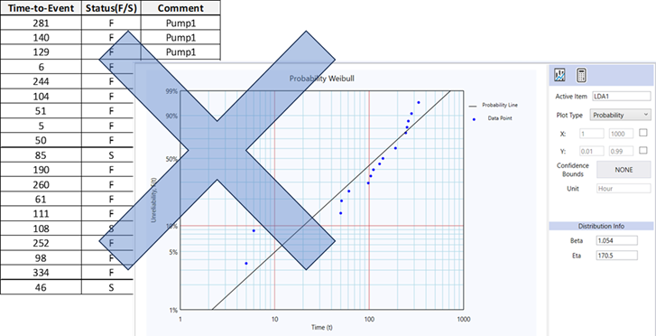
Why Fitting a Distribution Model to a Recurring Dataset Doesn’t Work? >
What are the limitations of LDA?
The requirement for identical and independently distributed (IID) data is essential in LDA. Each Time-to-Failure (TTF) data point should directly relate to a distinct physical item. However, in this instance, the time-between-failures doesn't align with the TTF of a physical item.
If we want to apply LDA to the pumps, we're constrained to considering only the time to the first failure to uphold the IID requirement. Consequently, we're left with only three data points. Moreover, dealing with subsequent failures poses a challenge.
Most failure history records obtained from CMMS or proprietary maintenance data logging systems often provide resolution details only up to the equipment level. Therefore, they primarily offer recurring information for analysis. As this type of data doesn't meet the IID requirement, using LDA for analysis becomes inappropriate.
What do want to know from the maintenance data?
- Predicting the expected number of failures for a given period of time, considering the current age of the equipment.
- Investigating whether there's statistical evidence indicating an increase in failure intensity (or decrease in Mean Time Between Failures) over time.
- Exploring the possibility of calculating the optimal overhaul time if the Mean Time Between Failures is decreasing.
An alternate approach is required to model recurring data effectively, enabling us to tackle these inquiries.
Recurring Data Analysis
The "Non-Homogeneous Poisson Process with Power Law" (NHPP/Power Law) stands as the predominant reliability model for recurring data. This model encompasses the Poisson Process and Power Law equations:
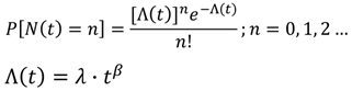
Here, P[N(t)=n] represents the probability of observing 'n' failures by time 't', while Λ(t) denotes the cumulative number of failures (Mean Value Function). The parameters λ and β within the equations are the model parameters to be determined.
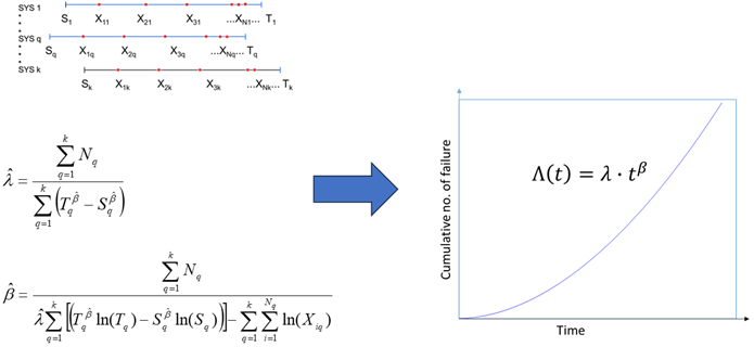
For this presentation, we utilized the Recurring Data Analysis tool in AeROS software to compute the model parameters λ and β. For a comprehensive understanding of the theory behind this analysis, consider exploring academic databases like PubMed, JSTOR, Google Scholar, or the IEEE Xplore Digital Library.
Figure 6 presents the recurring data from the three pumps, inputted into the RDA tool in a worksheet format.
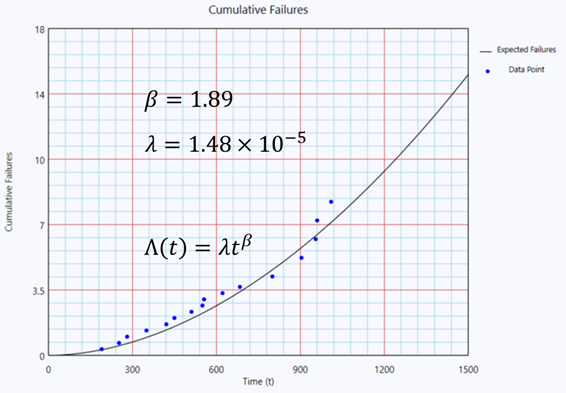
Utilizing the model parameters λ and β, the Mean Value Function Λ(t) is derived as illustrated:
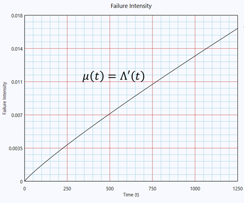
By taking the derivative of Λ(t), we acquire the failure intensity, denoted as µ(t) = Λ'(t), as shown in Figure 8.
Now, let's try to answer the following questions:
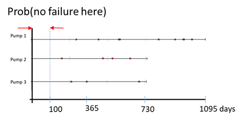
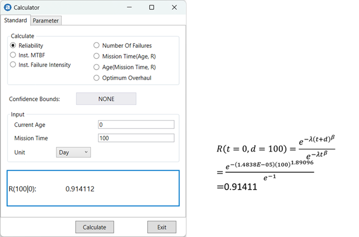
1. What is the probability that there is no failure in 100 days?
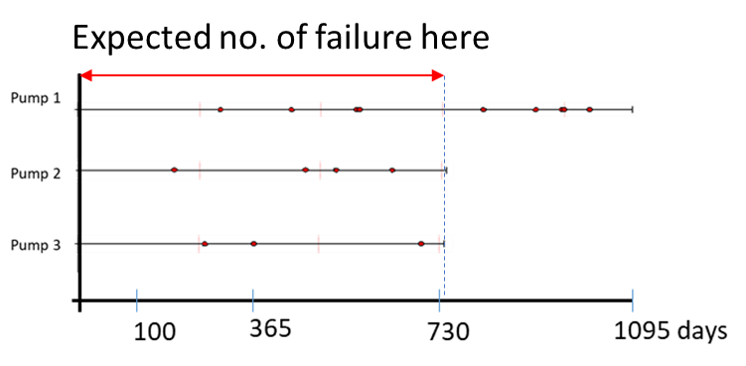
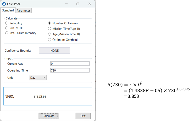
2. How many times will it fail within 2 years (730 days)?
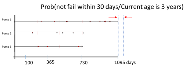
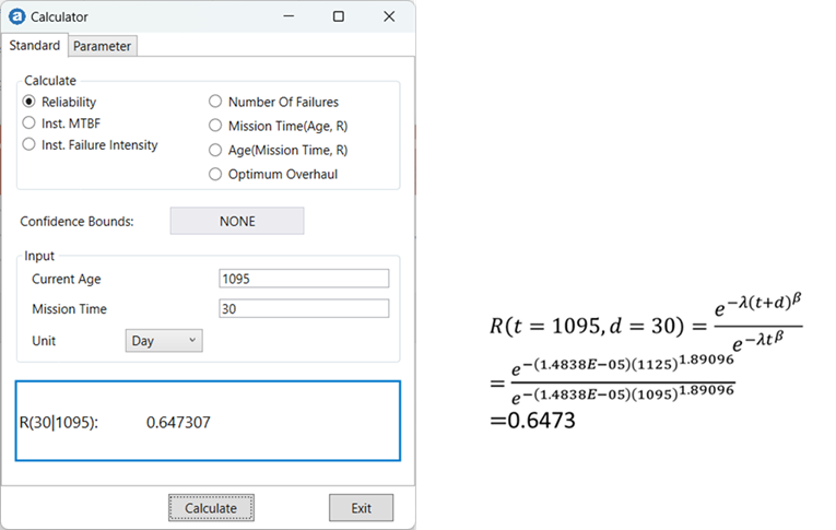
3. Given that system 1 is already 3 years old, what is the probability that it will not fail within the next 30 days?
Answers:
1. What is the probability that there is no failure in 100 days?
2. How many times will it fail within 2 years (730 days)?
3. Given that system 1 is already 3 years old, what is the probability that it will not fail within the next 30 days?
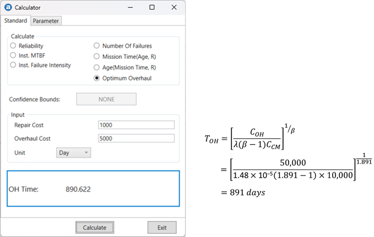
Optimum Overhaul (Economical Life)
From the failure intensity analysis, we can determine the optimum time to overhaul the system given repair and overhaul costs.
Conclusion
This presentation delineates the inappropriateness of Life Data Analysis (LDA) when dealing with recurring data, a common occurrence in failure data extracted from Computerized Maintenance Management Systems (CMMS) used by maintenance organizations. Instead, the recommended approach in such scenarios is Recurring Data Analysis (RDA).
RDA serves as a viable method to characterize the failure rate behavior of equipment or subsystems under the following circumstances:
- Data are not collected at non-repairable component level (LDA analysis is not feasible).
- Collecting equipment failure modes is not feasible due to the extensive effort required.
- You want to determine the optimum overhaul of a repairable equipment.
- You want to estimate reliability of a repairable equipment.
- You want to estimate expected number of failures a fleet of repairable system.
Related articles
Inventory Management: Forecasting Repairable Spare Requirements
Forecasting with Recurring Data Analysis: Risks and Limitations
- End -