A mining company has a policy to replace the lubricating oil of its fleet of machines when the oil TAN (Total Acid Number) value reaches a critical level. Recently, the engineer tested 2 brands on their machines.

Following are the Oil-Life-Before-Drain, in hours (Time-To-Failure) collected by the engineer.

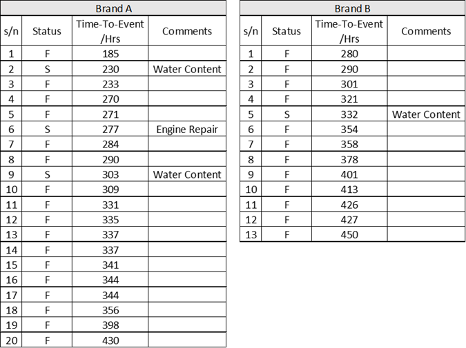
The TTF is obtained through monitoring the degradation of TAN content at a regular operating time interval, and the oil level is topped-up (with new oil) after the measurement if necessary.

When there is an engine failure, or the lubricating oil is found to have high water content, the oil will be completely drained. These data points are treated as suspension.

The company is currently using Brand A, and Brand B is the oil supplied by the competitor.

To replace oil for a machine with 130-gallon oil sump (bigger machines can have oil sumps up to 500 gallons) costs more than US$1,000. The Brand B manufacturer provided enough lubricating oil for 13 machines.

The engineer wished to know if there is any statistical justification to switch to Brand B.

The dataset is fitted to a 2-Parameter Weibull distribution with MLE setting:

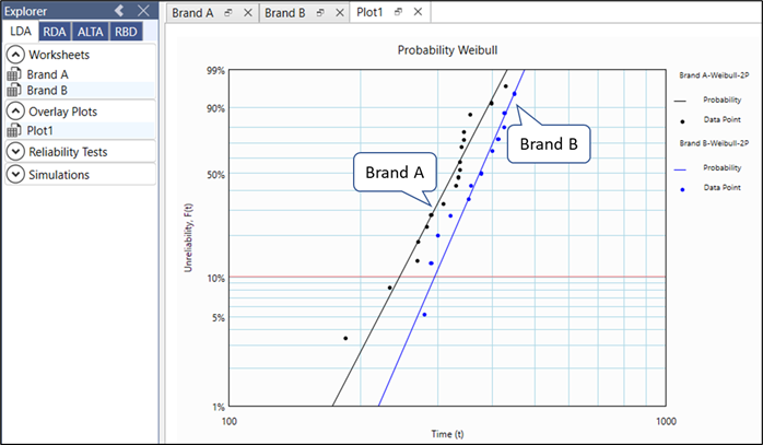
Life Data Analysis offers an elegant approach to comparing the reliability of products from different vendors.

The Weibull 2-Parameter distribution values are:

• Brand A: Weibull (Beta 6.644, Eta 343.8 hours)
• Brand B: Weibull (Beta 7.943, Eta 392.2 hours)

You can compare the Eta lifes using contour plots to check if they are significantly different.

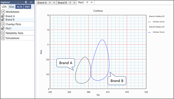
Since the contour plots do not overlap along Eta axis, we can say that the 2 brands are significantly different with 75% confidence.

Let's query the Mean Oil-Life-Before-Drain with the built-in calculator...

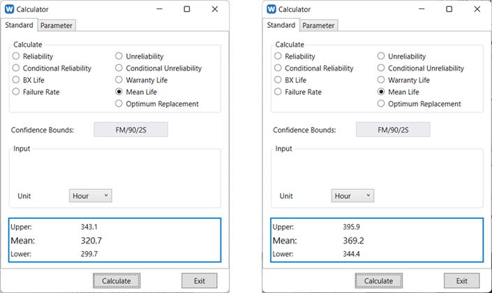
The Mean life (Mean Oil-Life-Before-Drain) with 90% confidence:

• Brand A: between 299.7 to 343.1 hours.
• Brand B: between 344 to 395.9 hours.

Assume the cost of both brands is the same - $1,000 for each oil change.

• The Mean Oil-Life-Before-Drain of Brand A and Brand B are 320.7 and 369.2 hours respectively. Hence, the oil running cost per hour for Brand A is $3.12 and Brand B is $2.71 per machine.
• Further assume that each machine accumulates 3,000 operating hours a year, the cost saving would have been 3,000 × (3.12 - 2.71) = $1,230 per machine (per year).
• Expected number of oil changes per year are 3,000/320.7 (or 9.35 times) and 3,000/369.2 (8.12 times) for Brand A and Brand B respectively. Potentially, a 12% reduction in labor cost associated with oil changing.
• In the case of 24/7 operations, the saving is even more significant. There will also be a saving due to lower downtimes i.e., an increase in availability.

From the above Life Data Analysis, Brand B has a significant cost benefit over Brand A, in terms of oil, labor and downtime costs.

The confidence bound calculated here does not reflect an inherent property of Brand A or Brand B but rather quantifies the uncertainty introduced by sampling variability. As expected, increasing the sample size reduces this bound, yielding greater precision in the results.

In this analysis, the dataset was sufficiently large to demonstrate a statistically significant difference between the two populations with 75% confidence.

Why Not a t-Test?

1. Normality Assumption – The t-test assumes that both groups follow an approximately normal distribution. However, most life data (e.g., reliability, survival, or time-to-failure data) deviate from normality, and assuming otherwise requires strong engineering judgment.
2. Equal Variance Assumption – The t-test also assumes homogeneity of variances (homoscedasticity), which cannot be confirmed in this case.
3. Censored Data Handling – Traditional t-tests cannot accommodate censored data (e.g., incomplete failure times), a common feature in life data analysis.

Advantages of Life Data Analysis

By leveraging this method, we avoid the restrictive assumptions of parametric tests while gaining clearer, more actionable insights into product reliability differences.

The Life Data Analysis approach overcomes these limitations, providing an elegant, robust, and intuitive solution. Its results are not only statistically sound but also highly visual, making them easier to interpret and communicate.