Consider an oil field with three unmanned oil production jackets, each containing an identical crude oil pumping system. Each system is equipped with two pumps—one operating and one on standby. A switching controller is also in place to automatically activate the standby unit if the operating unit fails.

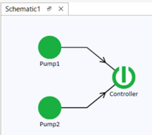
If the switching controller fails, it will not switch to the standby unit as required, leading to production loss for that jacket. However, the failure of the controller does not impact the overall pumping system's operation directly. This failure mode is classified as a hidden failure, meaning corrective maintenance (CM) for the controller will only be triggered during inspections or when it is discovered upon a failed attempt to activate the standby unit.

In this article, we assume the controller unit is a non-repairable component, meaning that any failed unit is replaced with a new one. For the pumps, we assume they are identical and operate with a common, constant failure rate.

Additionally, we assume that the maintenance downtimes are negligible compared to the system operating uptime in the subsequent discussions.

The following presents the failure timelines of three identical systems operating under the same production stress.

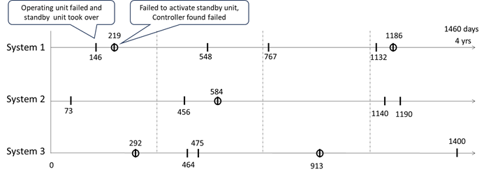
From these timelines, our goal is to extract the Time-to-Failure dataset for the controller unit to estimate its failure distribution.

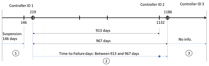
Controller ID 1: Failed at 219 days. No start date is available, but it operated for at least 146 days, making this a suspension data point: S(146 days). Controller ID 1 was then replaced with Controller ID 2.

Controller ID 2: Operated for at least 913 days, was found failed at 967 days, resulting in an interval data point: I(913, 967) days. Controller ID 2 was subsequently replaced with Controller ID 3.

Controller ID 3: There is no information indicating whether it was still operating up to day 1460.

From Figure 3, we derive two data points: one suspension data point, S(146), and one interval data point, I(913, 967).

Similarly, additional data points are derived from Systems 2 and 3, as illustrated in Figures 4 and 5, respectively.

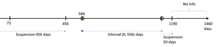
From Figure 4, three data points are derived: S(456), I(0, 556) and S(50).

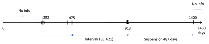
From Figure 5, two data points are derived: one interval data I(183, 621), and one suspension data S(487).

From the event timelines of the three systems, the following dataset was obtained (time in days):

• System 1: Suspension (146), Interval (913, 967)
• System 2: Suspension (456), Interval (0, 556), Suspension (50)
• System 3: Interval (183, 621), Suspension (487)

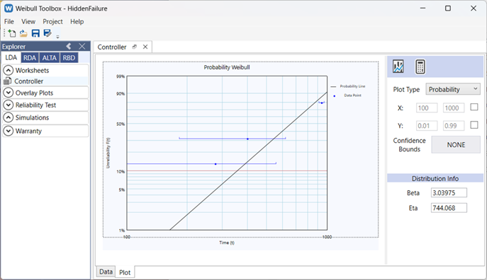
Note that, in most cases, datasets for hidden failure modes include suspension and interval data types. Maximum Likelihood Estimation (MLE) is suitable for heavily censored data, as seen here. The dataset was fitted using a 2-Parameter Weibull model.

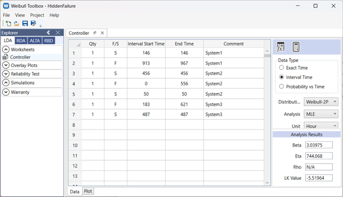
The operating life of the controller unit was estimated with a Weibull distribution, yielding a shape parameter, β = 3.04, and a scale parameter, η = 744 days.

Assume the following for all pumps in this analysis:

1. All pumps are identical.
2. Each pump has multiple failure modes, with a common constant failure rate.

Based on these assumptions, the pumps exhibit identical failure behaviour, which follows an Exponential life distribution. Thus, we only need to determine the Mean Time Between Failures (MTBF) for each pump.

Given that the total number of pump failures across 3 systems over 4 years is 16, hence, the average number of pump failures per system over 4 years is 16/3

Since only one pump operates per system at a time, the MTBF for each pump is calculated as:

MTBF = 4 years/ (16/3) = 0.75 years

This article demonstrated how failure data can be extracted from maintenance records for Life Data Analysis. For components with hidden failure modes, the dataset typically consists of right-censored and interval-censored data points.

For repairable assets with a stabilized failure rate, an Exponential life distribution is suitable. In these cases, calculating only the Mean Time Between Failures (MTBF) is sufficient to characterize the asset's reliability.

In the upcoming article, 'RAM Modeling with Hidden Failure Modes', we will explore methods to assess how the reliability of pump and controller units affects overall platform production.