Introduction

In this article, I will discuss how to analyze production impact due to supply (or input) variations using simulation approach.

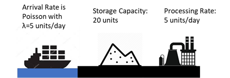
Consider the following scenarios: An iron ore receiving port takes in shipments and keeps it in a holding area. Meanwhile, the ore is consumed by nearby processing plant. If the holding area is full, new shipment cannot unload. When it is empty, production is interrupted. Both situations are not desirable.

In Operation Research, this type of problem is categorized under Queueing Theory.

For the purpose of this discussion, we normalize the quantity into some arbitrary unit. Each shipment delivers a quantity of 1 unit.

Assumptions

For simplicity, we will not include events due to, for example, failures of the conveyer system and the processing plant.

Shipment arrival variation can be described by Poisson process with λ = 5 shipments/day (or 0.2 day/shipments).
The holding area has a capacity of 20 units with 20% filled initially.
The plant processes the ore at the rate of 5 units/day, but it has a maximum processing rate of 6 units/day. It is designed to match the shipment arrival rate, and it does not fail in this example.

Figure 1: Processing plant relies on non-continuous supply

Unlocking Queueing Analysis Capabilities with AeROS™

Information Seeks

Understand the utilization of the holding area.
Minimize the interruptions to processing plant (when holding area becomes empty) and shipment operations (when holding area is full).

The Approach

A system model is created using AeROS software to simulate this scenario with the above requirements.

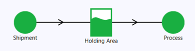
Figure 2: Simple process flow model with varying input

The Shipment node is configured to produce 1 unit with a mean time between arrivals of 0.2 days.

The Holding Area node (a specialized buffer/storage node) has a capacity of 20 units. It takes input from the Shipment node and outputs to the Process node simultaneously.

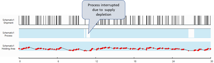
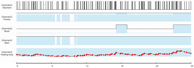
A 30-days simulation of 1000 executions is run, and the following shows the profile of a random execution:

Figure 3: Tri-state plot. Process node (Plant) interrupted due to ore supply depletion

The following is the simulation results for storage node (Holding Area):

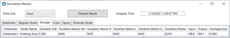
Figure 4: Simulation results for Holding Area storage node

Over 30 days, on the average, the Holding Area is:

Full for 5.6 hours
Empty for 26.6 hours

Note: When the Holding Area is full, shipments cannot unload. When it is empty, production is interrupted—both with potential cost implications.

In this model, the Process node operates at 5 units/day. We have not yet account for its maximum rate of 6 units/day.

Regulating Production Rate

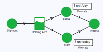
Figure 5: Manage Process node production rate by controlling the Boost Node rate

In Figure 5, we add a Boost Node to regulate the production rate. The Boost node is turned off (set to standby) so the production rate remains at 5 units/day during normal operation. The Holding Area is configured such that when its volume exceeds 50% of capacity, it activates the Boost node, increasing the Process node rate to 6 units/day. The Boost node returns to standby when the storage level drops to 25%.

A 30-days simulation of 1000 executions is run, and the following shows the profile of the last execution:

Process node operation — Figure 6: Process node normally processes 5 units/day. If storage exceeds 50%, increases to 6 units/day

The following shows the simulation results for storage node (Holding Area)

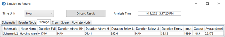
Over 30 days, on average, the Holding Area is:

Full for 0.17 hour, an improvement from 5.6 hours
Empty for 32.1 hours, getting worse compare to last configuration 26.6 hours

"What if" Analysis

Now, let's reconfigure the flowrates of the Boost and Main nodes to 2 and 4 units/day, respectively. This sets the Process node to operate at 4 units/day during normal operation.

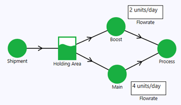
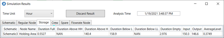
Flowrates configuration — Figure 8: Set the flowrates of Boost and Main nodes to 2 and 4 units/day respectively

Figure 9: Simulation results for Holding Area storage node

Over 30 days, on average, the Holding Area is:

Full for 0.5 hours
Empty for 3 hours

Using simulation, we can set up different scenarios to identify the most desirable operating procedures.

This method is also useful for proof-of-concept during early design stages.

Conclusion

Using the Storage node construct in AeROS software, engineers can analyze production impacts caused by supply (or input) variations. This analysis provides insight into the interactions among supply uncertainty, storage capacity, and operating procedures.

Although this case study focuses on supply variations, one could also add nodes with maintenance properties to model system reliability and analyze effects on production.

With some imagination, this analysis can be extended to include demand variations as well.

-End-