Introduction

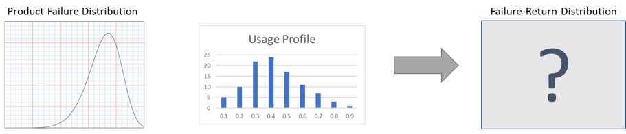
This example demonstrates how to predict field failure returns by combining accelerated lab test data with real-world customer usage profiles.

Using AeROS software, we simulate field-return distributions through:

Profile Nodes (an AeROS construct to model variable usage stress)
User-Defined CDFs (to represent usage profiles)
Time-To-First-Failure Simulation (to generate field failure data)

The results enable accurate warranty policy development by quantifying expected failure rates under actual usage conditions.

Figure 1: Estimate Failure-Return distribution from Product Failure distribution and Usage Profile

Input Data

Assumed an in-house test of an improved product demonstrates that its reliability follows Weibull distribution with beta=7, eta= 1000 hours. The test is conducted under constant, high usage rate in order to shorten the reliability test time. The usage stress level for the in-house test is arbitrarily set to 10 stress units/day.

The company conducted a field survey to determine the usage rate behavior of their customers for current product version.

The survey data is summarized as follow:

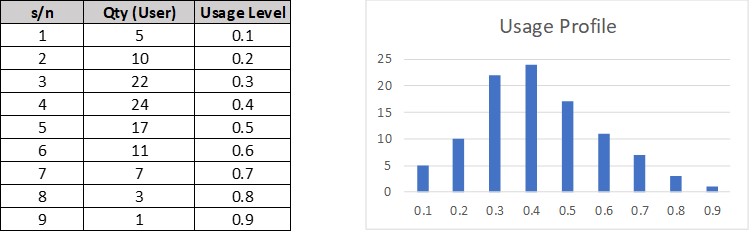
Figure 2: Usage profile obtained from survey data

Explanation:

row 1 : 5 users use 100 (10/0.1) times less frequent than in-house test (light-user).

row 9 : 1 user uses 11.1 (10/0.9) times less frequent than in-house test (heavy-user).

Information Seeks

The company wishes to determine the field failure distribution for the new product with this usage profile, and hence estimate the warranty returns on the first year for a given batch sold.

Methodology

This example uses user define discrete CDF to describe the Flowrate (usage) distribution. 200 random failure times (field-return failures) are generated through Time-To-First-Failure simulation in AeROS software. Life Data Analysis is applied to this Time-To-Failure dataset to obtain the field-return distribution.

Step 1: Create Reliability Digital Twin

A reliability digital twin is created using AeROS software.

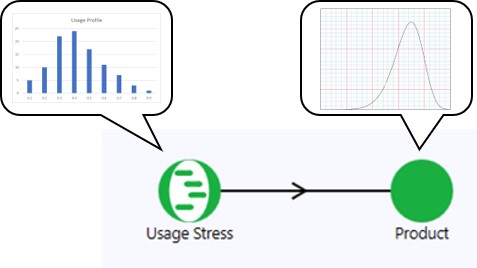
Figure 3: Profile Node 'Usage Stress' in series with a Regular Node 'Product'

Estimating Field Return Distribution Based on Reliability Test Results and Surveyed Usage Profiles.

The Product reliability followings Weibull distribution (Beta=7, Eta=1000 hours) at Design Flowrate (usage stress) = 10 units/day.

The Profile Node "Usage Stress" generates random usage level stress (Flowrate) based on usage distribution (to be defined in following section). The Product will fail according to its distribution with the reduced stress level (Flowrate). This process is repeated to generate field-return dataset.

This example assumes that the in-house test was a usage-rate-accelerated test. A user in the field is expected to use the product at lower usage rate. This means if the Flowrate (usage rate) reduces from 10 to 1 unit (10 times), the product life increased by 10 times.

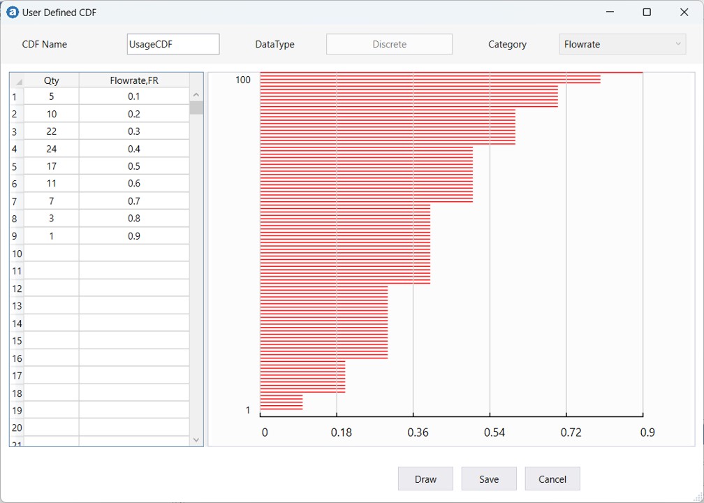
Step 2: Model Usage Variability (Usage Stress Profile)

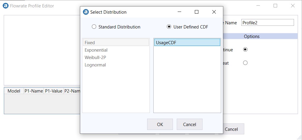
The first step is to create a discrete user-defined-CDF, and then apply it to the Flowrate Profile of Usage Stress (Profile Node).

A discrete user-defined-CDF is created using the survey data.

Figure 4: The Usage Profile is defined as discrete Cumulative Density Function (CDF)

Step 3: Configure Flowrate Profile

The next step is to create a Flowrate Profile (a property of Profile Node "Usage Stress" node) that contains only one segment which in turn define flowrate distribution and duration.

The Flowrate Profile Editor is used to create Flowrate Profile.

The flowrate profile is made up of N segments (where N > 0). Each segment defines a flowrate distribution (or a fixed value) and a duration. The time unit is defined when you associate this profile to a Profile Node later (See Fig.7).

"UsageCDF" is assigned the first and only segment of this Flowrate Profile.

Figure 5: Select 'UsageCDF' as the only segment for Flowrate Profile

Flowrate Profile Editor displays the flowrate profile.

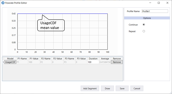
Figure 6: The Flowrate Profile contains only one segment defined by 'UsageCDF'

The vertical axis shows the mean flowrate value of each defined segment. In this case, there is only one segment. This segment flowrate mean value is 0.42, and duration is 100 units time (default value, and the time unit is defined at the Profile Node later). After 100 units time, the Flowrate will remain, since "Continue" option is selected.

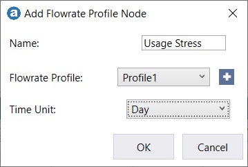
Note that the default Profile Name is "Profile1".

The next step is to create Profile Node "Usage Stress" and assign Flowrate Profile "Profile1" to it.

A Profile Node is added to the schematic with Duration Unit set to Day and renamed it to "Usage Stress"

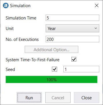
Figure 7: Associate Flowrate Profile 'Profile1' to Profile Node

Step 4: Simulate Field Failures

After defining the usage-stress profile and the product failure distribution parameters, we ran a simulation to generate 200 field-return data. These are later analyzed using Life-Data Analysis (Figure. 10).

Figure 8: Using simulation to generate 200 data points using 'System Time-To-First-Failure' option

The Time-To-First-Failure Plot shows the simulation results.

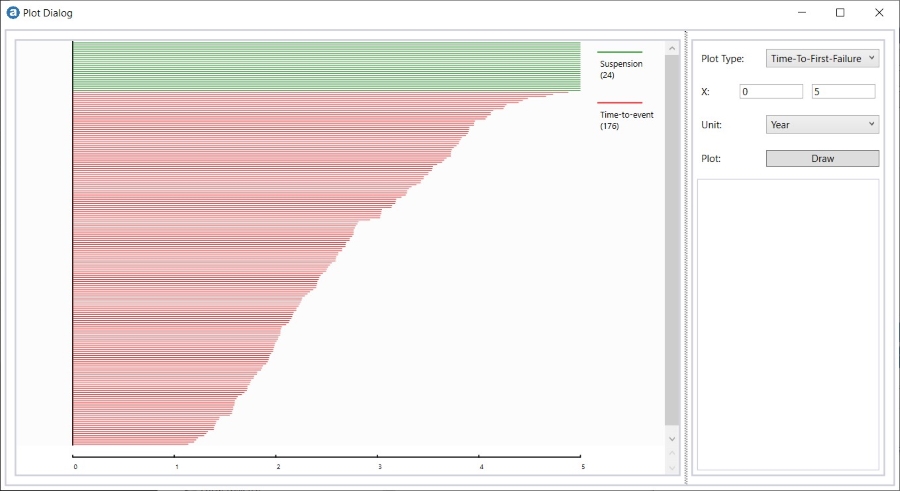
Figure 9: Visualization of the sorted 200 data points

The red and green lines represent the Time-To-Failures and Suspensions respectively.

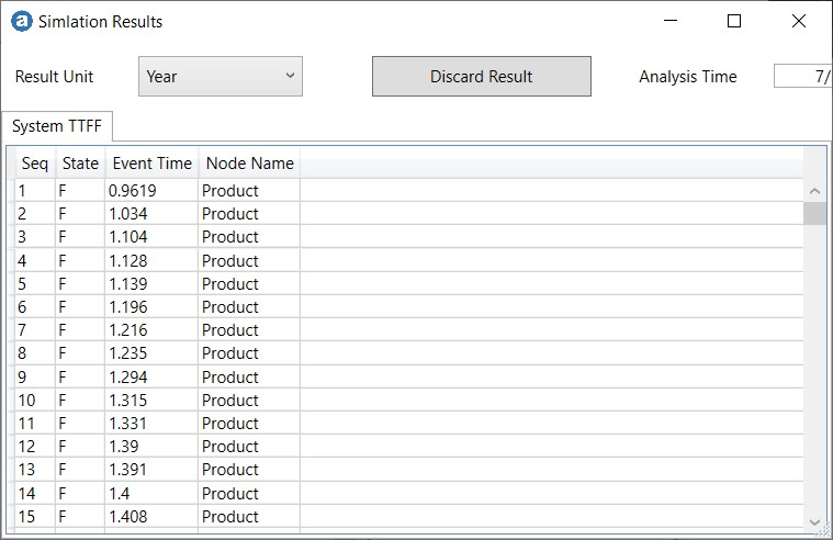
Following is the Time-To-Failure/Suspension data in data-grid format.

Figure 10: Generated data points in data-grid format

Results

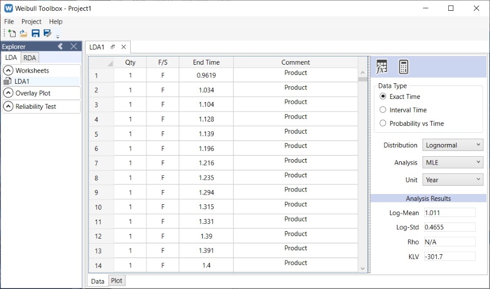
The dataset is transferred to Worksheet in Weibull Toolbox software, and fitted with Lognormal distribution using MLE analysis:

Figure 11: Performed Life-Data-Analysis on the generated data

Followings are the Probability and PDF plots:

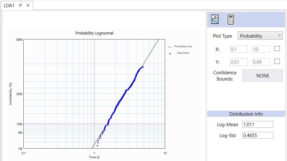
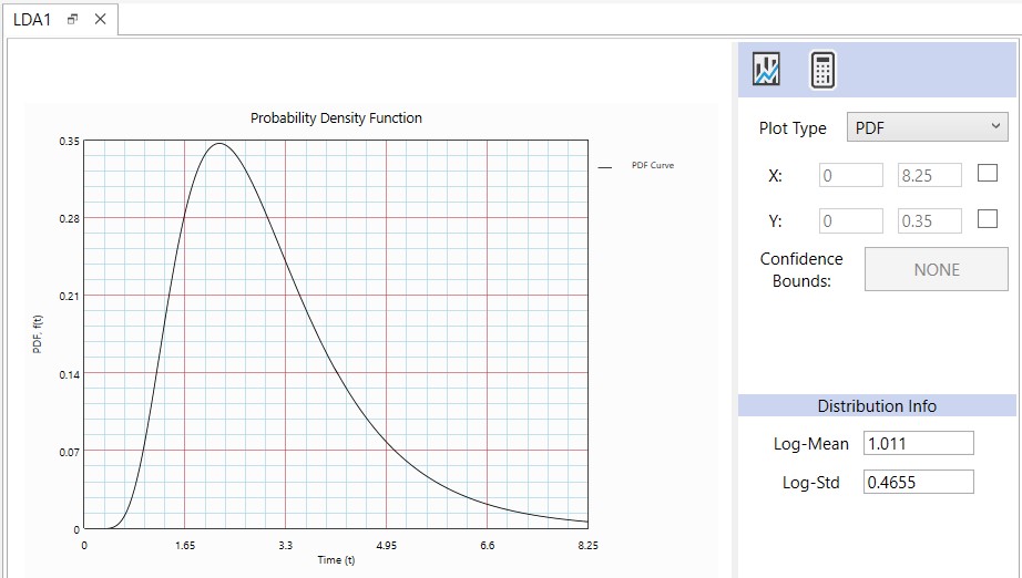
Figure 13: Probability Density Function plot

The failure rate behavior is estimated with Lognormal (Log-Mean = 1.011/year, Log-Std 0.4655) distribution

The percentage of failure-returns one year after a batch is sold can be determine as shown:

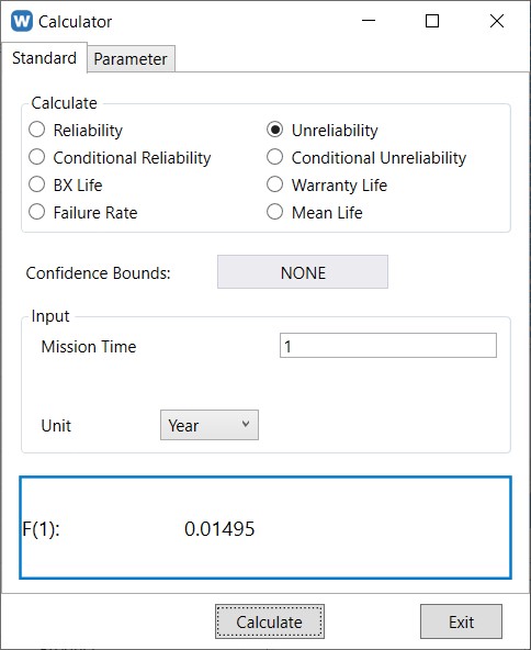
Figure 14: Probability of failure at first year, Q(1 year) = 0.015

For a batch of 10,000 units, ~150 returns are expected within Year 1.

Conclusion

This example illustrates how lab reliability test data and usage profile information can be combined to generate field-return distributions, which serve as a foundation for estimating warranty returns.

-End-